Single-point calculation#


Click on the Parameters icon to open the Single-point Parameter widget,
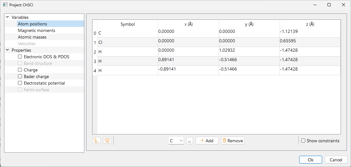
Please refet to the Variables section to know how to edit Atomic positions, Magnetic moments, Atomic masses and Velocities in ASAP.
When Single-point calculation is selected the user can decide to compute additional properties, please refer to the section Properties for a detailed explanation.
Click on the Calculator icon to select the computational engine to be used during the single point calculation.


Analysis#
The information provided by the analysis widget also depends on the properties that were selected on the Parameters widget, see section Properties.
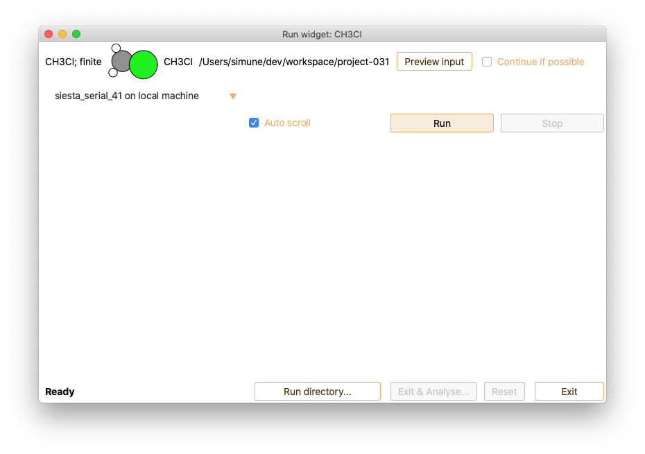
When the calculation is completed, press the Exit and analyse button to open the single-point analysis widget.

The following information extracted from the single-point calculation output is available:
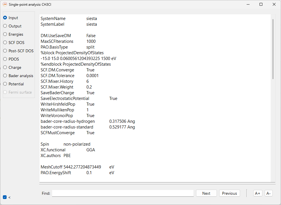
Input#
It shows the complete input file of the single-point calculation. This option is only available for SIESTA calculator.
Output#
It shows the complete output file of the single-point calculation.

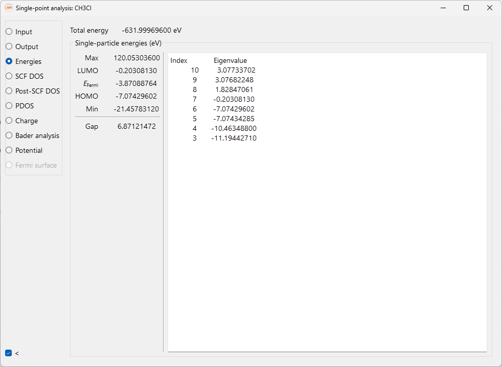
Energies#
It shows the information on: Total energy, Fermi energy minimum, maximum and frontier orbital energies HOMO (highest occupied molecular orbital) and LUMO (lowest unoccupied molecular orbital). As well as energy gap and Eigenvalue energies.
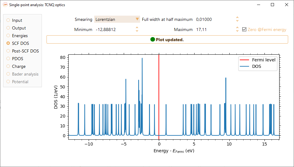
Density of States#

Smearing. Gaussian or Lorentzian representations of the Dirac delta function.
Full width at half maximum (FWHM) The broadening is defined by the full-width-at-half-maximum in both representations (Gaussian and Lorentzian) of the Dirac delta function.
Zero @ Fermi. Sets the origin of the DOS function at Fermi level.
Right-click on the density of states figure to make available the following options:
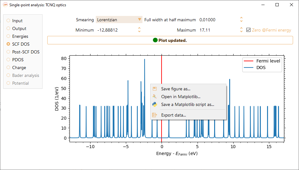
Save figure as…. We support the following formats: pdf, png, jpg, jpeg, ps, eps, and svg.
Open in Matplotlib… Open with Matplotlib the python script used to plot the figure.
Save a Matplotlib script as… Save the python script used to plot the figure.
Export data… Export the data from the density of states figure to a text file format.
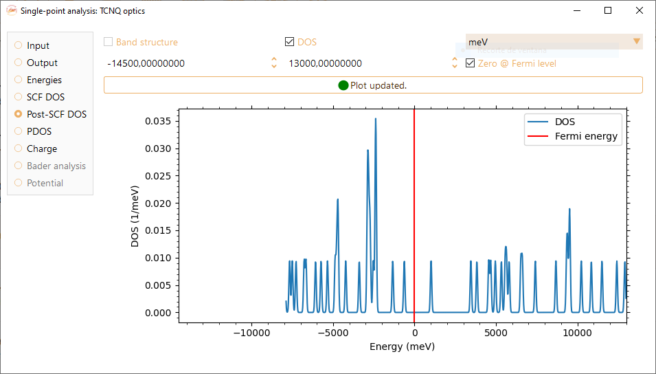
Check the Post-SCF-DOS tick box to visualize the density of states computed after a self-consistent field loop with a custom BZ sampling.

You can adjust the energy range (x-axis) by tuning the minimum and maximum energies shown at the top of the widget, in units of eV, meV, kcal/mol, kJ/mol, Ha, mHa, Ry and mRy.

Check the Zero @ Fermi level tick box to set the origin of the post-SCF DOS function at the Fermi energy level.
The electronic band structure of a solid describes the range of energies that an electron within the solid may have (energy bands) and the ranges of energies it may not have (band gaps). Check the Band structure tick box to visualise the corresponding graph. Please note that this option is only available for infinite-sized systems.

Notice that you can adjust the band structure energy range (y-axis) by tuning the minimum and maximum energies shown at the top of the figure, in units of eV, meV, kcal/mol, kJ/mol, Ha, mHa, Ry and mRy.
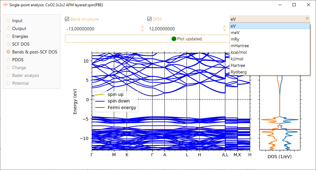
Check the Zero @ Fermi level tick box to center the DOS at the Fermi energy level.

Right-click on the band structure figure to make available the following options:

Save figure as…. We support the following formats: pdf, png, jpg, jpeg, ps, eps and svg.
Open in Matplotlib…. Matplolib library allows the user an interactive visualisation of the figure (scale axis, zoom on speci1c X and Y values…).
Save a Matplotlib script as…. Save the Matplotlib script used to plot the figure.
Export band structure to JSON…
Export band structure to .bands…
Export DOS…. Export the data from the band structure figure to a text file format.
Partial DOS#
Check the PDOS option to visualise the partial density of states of the system.
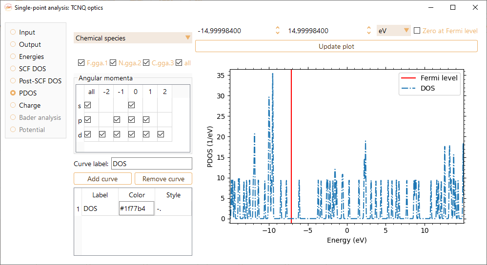
To visualise the projected DOS on specific atoms, select them by their chemical species or choose a range of atom indices.

You can also select the angular momenta of the atomic orbitals that will be included in the PDOS visualisation.

You can change the label at your convenience. Press the Add curve button to incorporate each of your selections.

You can change units on the top right side of the widget. The options are eV, meV, kcal/mol, kJ/mol, Ry, mRy, Ha and mHa.


You can change the colors of the curves by tuning the value on the Color column in the table on the bottom left of the widget. Please note that you must use Hexadecimal code.
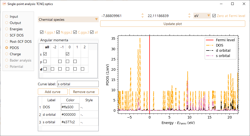
Additionally, you can change the style of the lines by tuning the value on the column Style on the bottom left of the widget. Supported values are ‘-’, ‘–’, ‘-.’, ‘:’, ‘None’, ‘ ‘ , , ‘solid’, ‘dashed’, ‘dashdot’, ‘dotted’.

Charge#

You can visualise the charge of each atom of the project calculated by the selected methods. These charges are given in units of electrons.
Bader analysis#
When the project is successfully completed, click the Exit & analyse button.

Then select Bader analysis in the Analysis widget.

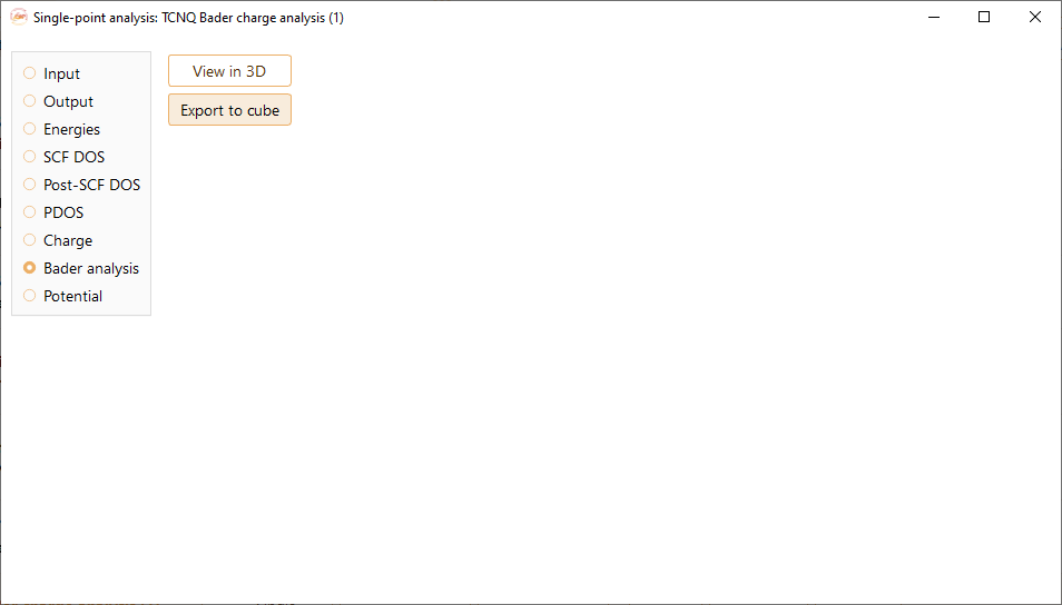
Click the View in 3D button to view the structure in the advanced 3D viewer. You can see the equipotential surface induced by the charge distribution for a determined isovalue. See section Advanced 3D viewer for further information on the 3D advanced viewer.
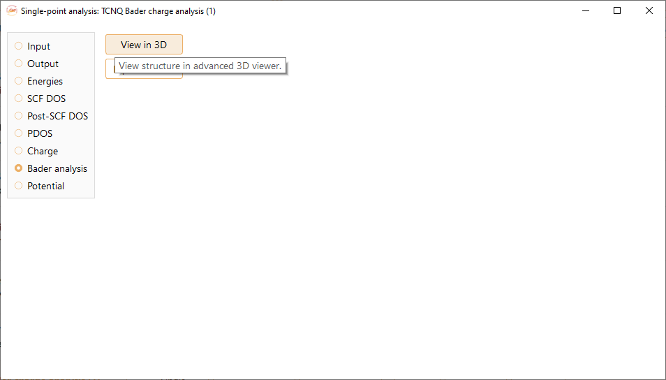

In the previous figure you can see the structure of the project in 3D and the Bader charge isosurface.
Press the Export to cube button to export the volumetric data of the Bader analysis to a cube file.
Electrostatic potential#
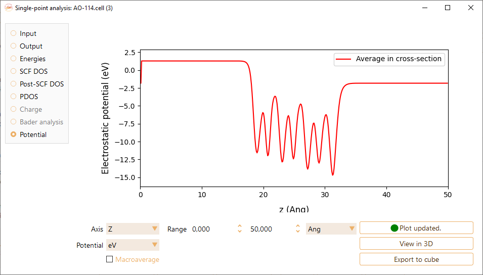

Axis: The axis (X, Y or Z) in which the electrostatic potential is evaluated.
Potential: The units of the electrostatic potential: eV, meV, Rydberg or Hartree.
Range: The range used as the x-axis. The units can be Å, Bohr and nm.


Fermi Surface#
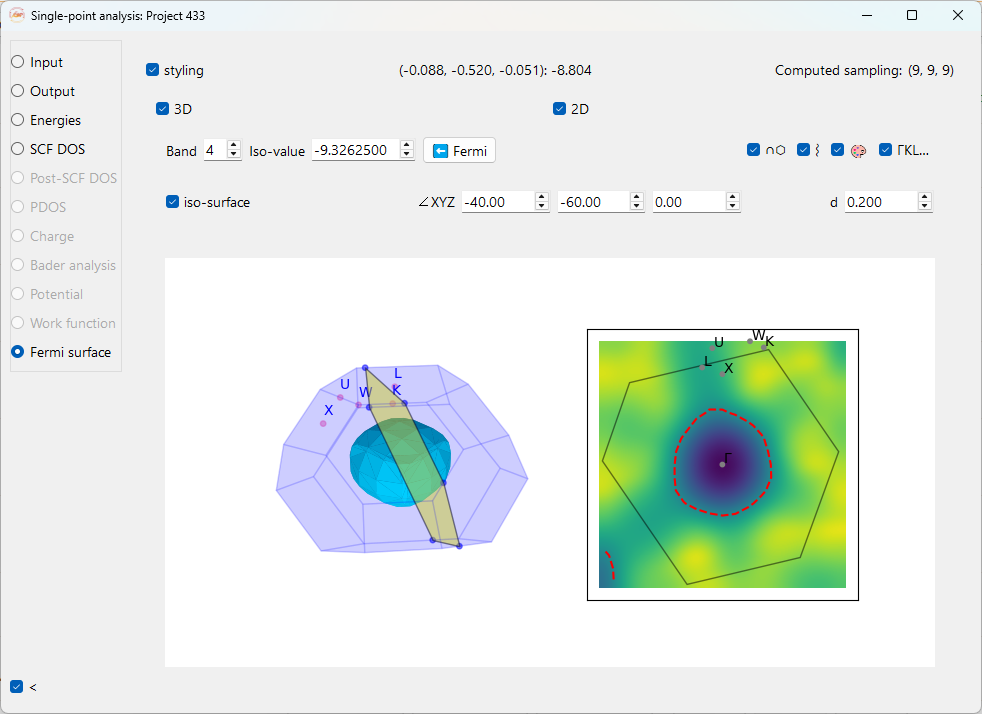
Panel Header Information
Coordinates and Value: Clicking on the 2D plot displays the k-point fractional coordinates and the corresponding energy (in eV) at that point.
Computed sampling: Non-editable field that displays the k-point sampling grid (e.g., (9, 9, 9)) used to generate the data for the Fermi surface.
Editable Parameters (top row)
styling: Check this checkbox to toggle the visibility of advanced styling options for the plots.
3D: Toggles the display of the 3D Fermi surface visualization in the left-hand panel.
2D: Toggles the display of the 2D Fermi surface cross-section in the right-hand panel.
∩⬡: Show the plane intersecting Brillouin zone at the angles defined by ∠XYZ and d.
⌇: Show the isoline for the selected isovalue in the 2D plot when checked.
🎨 : Show the colormap on 2D plot when checked.
ΓKL… (High symmetry k-points): This button displays the high symmetry k-points labels on the 2D and 3D plot.
Editable Parameters (second row)
Band: Use this dropdown menu to select the specific electronic band for which to plot the isosurface. You can select different bands to see their individual contributions to the Fermi surface. Press the Enter key to update the plot.
Iso-value: This field allows you to manually set the energy (in eV) for which the isosurface is plotted. Press the Enter key to update the plot.
Fermi: Click this button to automatically set the band and iso-value to the calculated Fermi energy of the system.
iso-surface: Check this checkbox to show or hide the 3D isosurface plot.
∠XYZ: These three fields are the Angles in degrees (°) that define the orientation of the 2D plane intersecting the Brillouin zone.
d: This field sets the distance in the reciprocal space in Angstrom (\(\text{Å}^{-1}\)) of the 2D plane from the Γ-point (the origin of the Brillouin zone). A value of 0.000 means the plane passes through the center.
3D and 2D Plots
Click and hold the left mouse button on the 3D plot to rotate it for better visualization.
Use the right mouse button and drag the mouse forward or backward to zoom in and out of the 3D plot.
Single left click on the 2D plot to display the reciprocal fractional coordinates and the corresponding energy value (in eV) at that point.
Double left click to set a new isovalue.