Molecular Dynamics#


The settings widget associated with a MD type of project offers the following options:
- t-step. This parameter controls the length of the time step in the MD simulation. If the time step is too large, the dynamics of the system will show unphysical non-energy conservation behavior, population of high-frequency modes, even melting. Therefore, if the system includes light atoms as Hydrogen, it is necessary to consider a reduced time step. It is always safer to choose a small time step. However, this will increase computation time. We advise examining the system under study and select the time step carefully. For most metallic systems, a time step of 5 fs would be a good choice. Systems with light atoms (e.g. hydrogen), and/or with strong bonds (e.g. C-C, C-H) will require a smaller time step.The time units are selected at the rigth of this parameter. The options are femto-seconds (fs), i.e. 10\(^{-15}\) seconds, and pico-seconds (ps), i.e. 10\(^{-12}\) s.
n steps. Number of steps of the MD simulation. The number of steps multiplied by the time step will give a full-time MD calculation.
Logging frequency defines how frequently the information of a running MD calculation is stored. During the MD simulation, atomic positions and velocities are stored. This is very useful to visualise and analyse the calculations.
Algorithm. ASAP currently has different statistical ensembles integrated by the following algorithms:
Verlet (NVE): Standard Verlet algorithm. Microcanonical ensemble, where the number of atoms (N), volume (V) and total energy (E) are conserved.
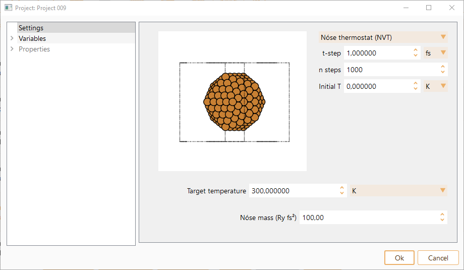
Nosé thermostat (NVT): MD with temperature controlled by means of a Nosé thermostat. Only available for MD-SIESTA
Parrinello-Rahman (NP): MD with pressure controlled by the Parrinello-Rahman method. Only available for MD-SIESTA
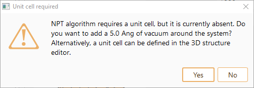
Nosé Parrinello-Rahman (NPT): isothermal–isobaric ensemble, where the number of atoms (N), pressure (P) and temperature (T) are conserved. MD with temperature is controlled by means of a Nosé thermostat and pressure controlled by the Parrinello-Rahman method.
Annealing. MD with annealing to a desired temperature and/or pressure. Only available for MD-SIESTA
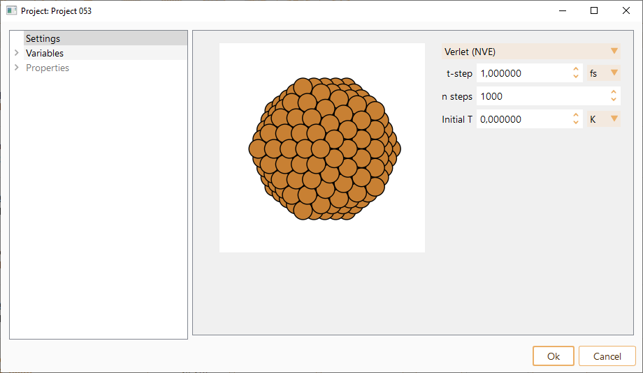
Initial T. Initial temperature for the MD run. Represents the intial kinetick energy distribution of the particles. The atoms are assigned random velocities drawn from the Maxwell-Bolzmann distribution with the corresponding temperature. The constraint of zero center of mass velocity is imposed. In units of K, eV or meV.
Initial T. Initial temperature for the MD run. The atoms are assigned random velocities drawn from the Maxwell-Bolzmann distribution with the corresponding temperature. The constraint of zero center of mass velocity is imposed. In units of K, eV or meV.
Target temperature. Target temperature for Nosé thermostat. In units of K, eV or meV.
Nosé mass. Generalised mass of Nosé variable. This determines the time scale of the Nosé variable dynamics, and the coupling of the thermal bath to the physical system.

Initial T. Initial temperature for the MD run. The atoms are assigned random velocities drawn from the Maxwell-Bolzmann distribution with the corresponding temperature. The constraint of zero center of mass velocity is imposed (in units of K, eV or meV).
Target pressure. Target pressure for Parrinello-Rahman method. In units of GPa, eV/Angström\(^{3}\) or Ry/Bohr\(^{3}\) .
Parinello-Raman mass. Generalised mass of Parrinello-Rahman variable. This determines the time scale of the Parrinello-Rahman variable dynamics, and its coupling to the physical system.

Temperature. In units of K, eV or meV.
External stress. In units of eV/Angström\(^{3}\) or GPa.
T-time. Frequency of the temperature updates (in units of fs).
P-time. Frequency of the pressure updates (in units of fs).
B-mod. Bulk modulus. Measures a material’s resistance to uniform compresion (in units of eV/Angström\(^{3}\) or GPa).

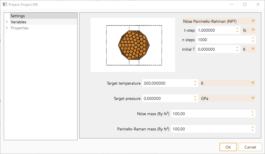
Initial T. Initial temperature for the MD run. The atoms are assigned random velocities drawn from the Maxwell-Bolzmann distribution with the corresponding temperature. The constraint of zero center of mass velocity is imposed. In units of K, eV or meV.
Target temperature. Target temperature for Parrinello-Rahman method. In units of K, eV or meV.
Target pressure. Target pressure for Parrinello-Rahman method. In units of GPa, eV/Angström\(^{3}\) or Ry/Bohr\(^{3}\).
Nosé mass. Generalised mass of Nosé variable. This determines the time scale of the Nosé variable dynamics, and the coupling of the thermal bath to the physical system.
Parinello-Raman mass. Generalised mass of Parrinello-Rahman variable. This determines the time scale of the Parrinello-Rahman variable dynamics, and its coupling to the physical system.

If the Temperature is selected, the additional settings are:
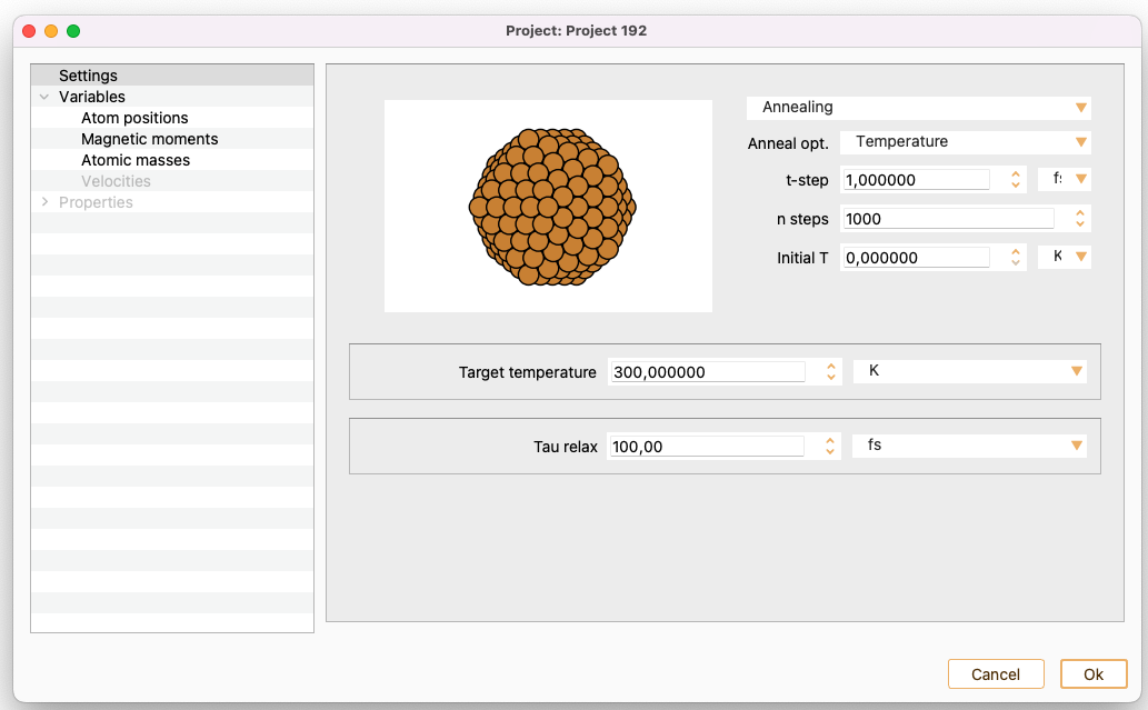
Target temperature. Target temperature for annealing MD. In units of K, eV or meV.
Tau relax. Relaxation time to reach target temperature and/or pressure in annealing MD. Note that this is a relaxation time, and as such it gives a rough estimate of the time needed to achieve the given targets. As a normal simulation also exhibits oscillations, the actual time needed to reach the averaged targets will be significantly longer.
If the Pressure is selected, the additional settings are:

Target pressure. The target pressure is achieved by velocity and unit cell rescaling, in a given time determined by the variable Tau relax. In units of GPa, eV/Angström\(^{3}\) or Ry/Bohr\(^{3}\).
Bulk modulus estimation. Estimation (may be rough) of the bulk modulus of the system. This is needed to set the rate of change of cell shape to reach target pressure. In units of GPa, eV/Angström\(^{3}\) or Ry/Bohr\(^{3}\).
Tau relax. Relaxation time to reach target temperature and/or pressure in annealing MD. Note that this is a relaxation time, and as such it gives a rough estimate of the time needed to achieve the given targets. As a normal simulation also exhibits oscillations, the actual time needed to reach the averaged targets will be significantly longer. In units of fs and ps.
If both Temperature and Pressure are selected, the additional settings are:

Target temperature. The target temperature is achieved by velocity and unit cell rescaling, in a given time determined by the variable Tau relax. In units of K, eV or meV.
Target pressure. The target pressure is achieved by velocity and unit cell rescaling, in a given time determined by the variable Tau relax. In units of GPa, eV/Angström\(^{3}\) or Ry/Bohr\(^{3}\).
Bulk modulus estimation. Estimation (may be rough) of the bulk modulus of the system. This is needed to set the rate of change of cell shape to reach target pressure. In units of GPa, eV/Angström\(^{3}\) or Ry/Bohr\(^{3}\).
Tau relax. Relaxation time to reach target temperature and/or pressure in annealing MD. Note that this is a relaxation time, and as such it gives a rough estimate of the time needed to achieve the given targets. As a normal simulation also exhibits oscillations, the actual time needed to reach the averaged targets will be significantly longer. In units of fs and ps.

The initial velocities are initially set to zero, however, they can be changed manually. The constraint on zero center of mass velocity is imposed automatically. Random velocities drawn by a Maxwell-Boltzmann distribution can be assigned to atoms of the system. You can set a desired temperature in the Maxwell-Boltzmann box. Press the Initialize now button to set up the initial velocities.

To maintain the system at the target temperature select the Force tick-box.


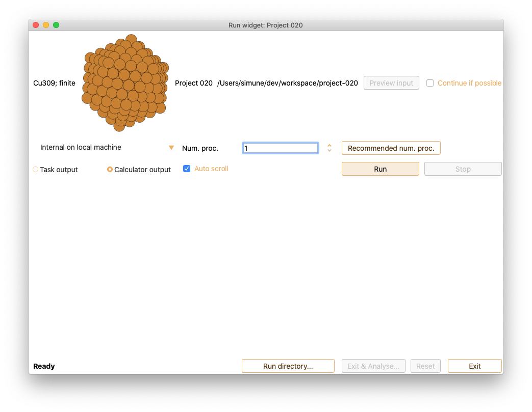
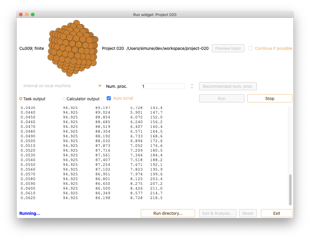
After submitting a job (run), the Calculator output tab in Run widget shows the complete calculation output in real time. In addition, the Task output tab in Run widget shows relevant information on the Molecular Dynamic output in real-time.
Analysis#


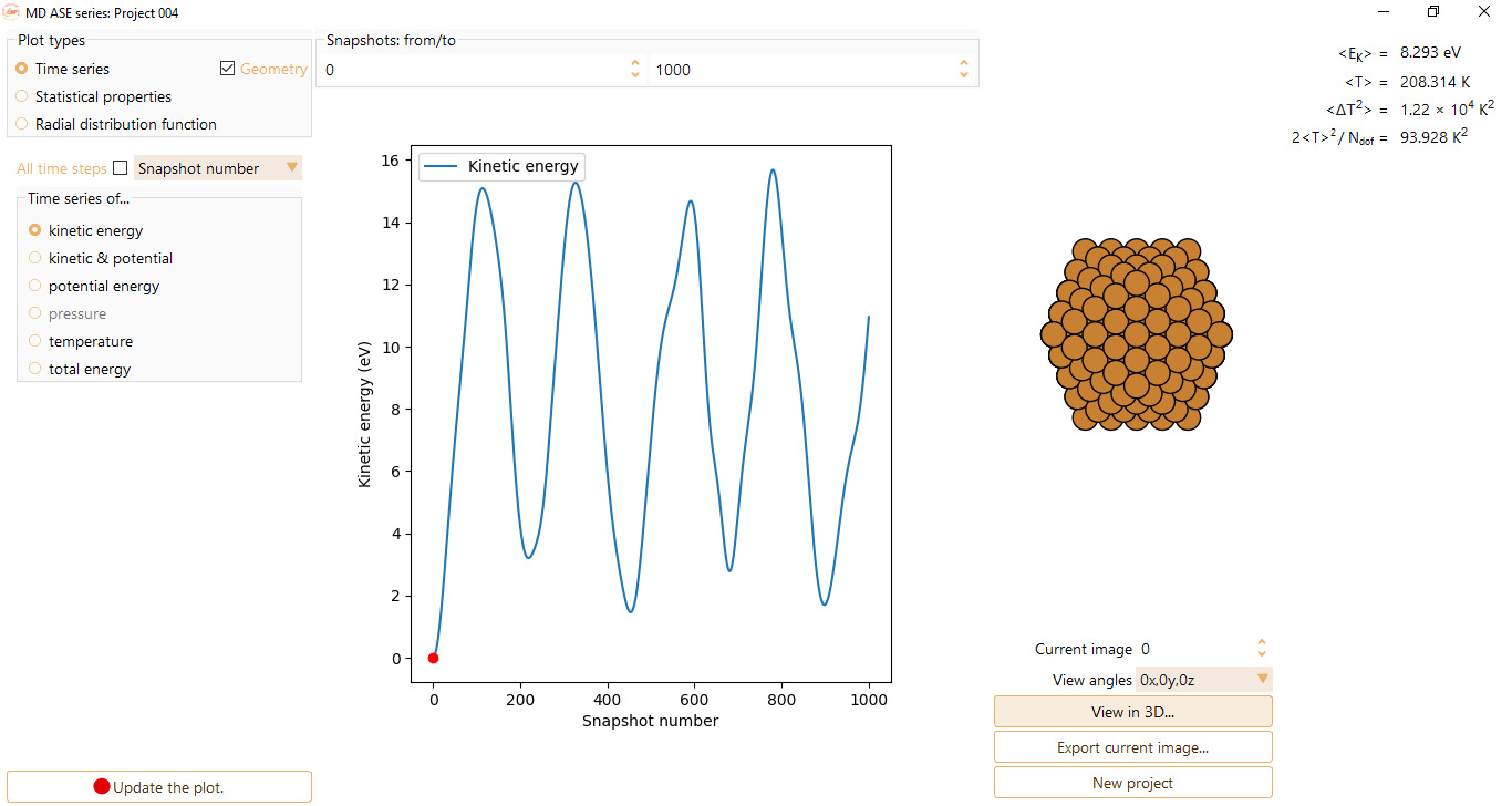
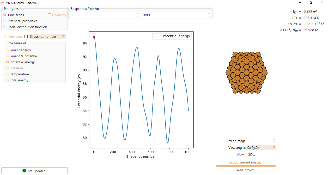
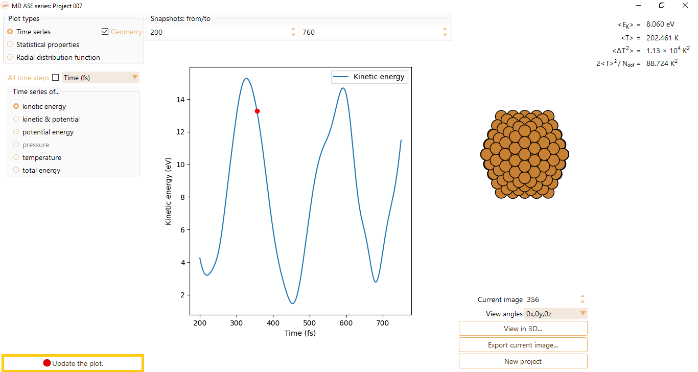
\(\langle Ek \rangle\) and \(\langle T \rangle\) are the average kinetic energy and average temperature, respectively. These parameters are helpful to control the evolution of the system during dynamic run.
\(\langle \Delta T^{2} \rangle\) represents the average temperature variation observed during an MD run. This parameter provides insight into the magnitude of temperature fluctuation that occur throughout the simulation. This measurement is particularly valuable for analyses conducted near phase transitions, as it effectively captures significant fluctuations that often manifest in such scenarios.
2\(\langle T \rangle^{2}\)/N is the averaged square temperature normalised by the degrees of freedom (N). It is an indirect measure of specific heat.
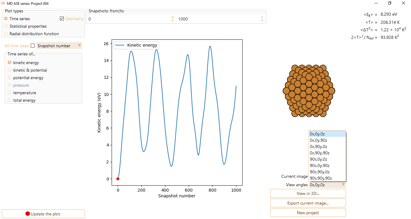
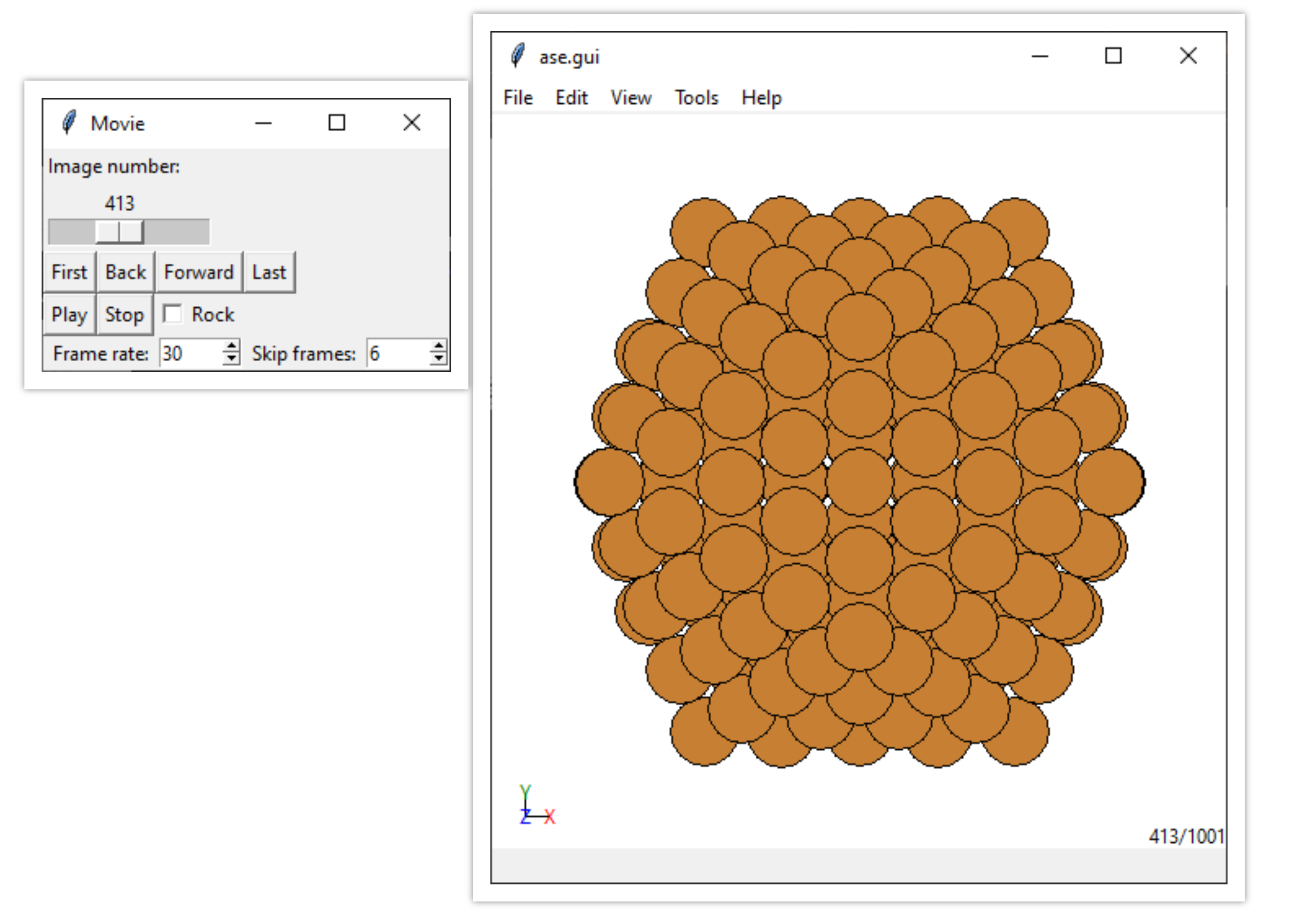
Press the View in 3D… button to visualise the image with ASE GUI at the selected step.
Press the Play button to visualise the structure’s evolution during the MD run in three dimensions.
You can visualise the results of MD as time series (y-axis) of:
kinetic energy

kinetic and potential. For the visualisation of both kinetic and potential energies.

potential energy
pressure. The option is only available if provided by the calculator.
temperature.

total energy

Notice that you can modify the logging step range that will be shown in the visualisation,

and visualise the Time series as a function of steps or time (in unit of fs).
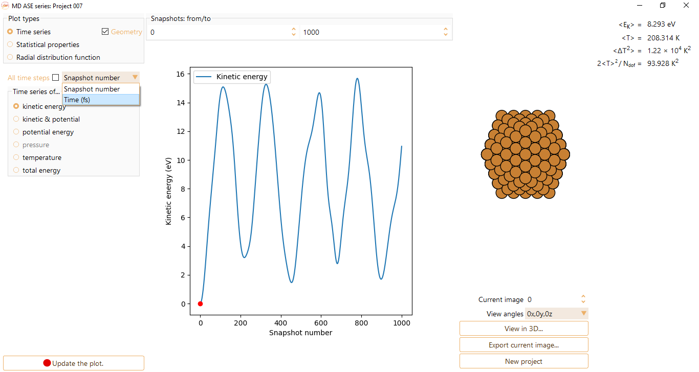
After editing a parameter, click the Update the plot button.
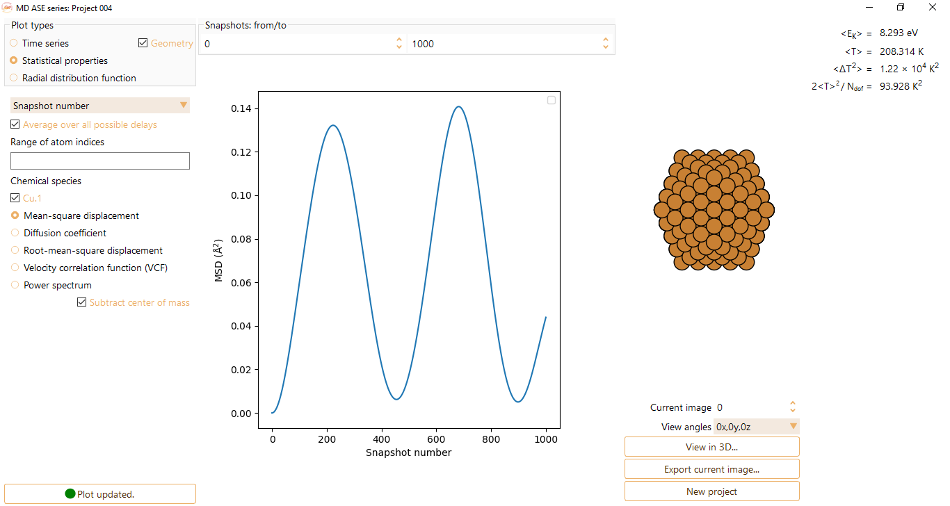
Mean-square displacement: The average square distance taken over all particles. Gives the deviation of the position of a particle with respect to a reference position over a certain period of time (units of Angström\(^{2}\)).
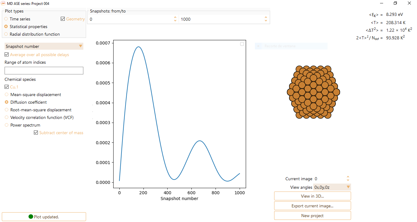
Diffusion coefficient: Amount of substance passing through a certain boundary per unit area and per unit time (units of Angström\(^{2}\)/fs).
Root-mean-square displacement: measures the variability of the positions of the particles with respect to a reference position over a certain period of time. It is particularly useful to compare two data sets of a system that has been transformed in some way (units of Angström).

Velocity correlation function (VCF): average of the product of the velocities of all the particles at two different times (t, t+\(\Delta\)t). This function quantifies the rate at which the particles return to equilibrium state after a small perturbation.

Power spectrum: allows the user to visualize the frequency distribution of the velocity correlation function (units of fs). It helps to identify characteristic frequencies and modes of vibration of the system. Note that for this statistical property the options for the abscissa axis are not steps or (explicitly) time, but frequency as a function of time (units of fs) or inverse of time (Hz), inverse of wavelength (units of cm-1) and energy (units of eV, meV, and Rydberg and Hartree units of energy).

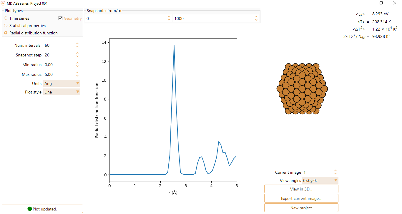
You can tune the following parameters:
Num. intervals: parameter defining the sampling of the x axis.
Snapshot step: to select a specific moment in time of the MD run.
Min radius: minimum radial distance for the RDF.
Max radius: maximum radial distance for the RDF.
Units: optionally units of Angström, nanometers or or Bohr radius.
Plot style: optionally lines or bars.
