Optical response

With this type of project, you can calculate the optical properties of a system; real and imaginary part of the dielectric function. The approach used is based on computing the dipolar transition matrix elements between different eigenfunctions of the self-consistent Hamiltonian. For molecules, the calculation is performed using the position operator matrix elements, while for solids, the calculation is carried out in the momentum space formulation.

Corrections due to the non-locality of the pseudopotentials are introduced in the usual way.

The project starts with the definition of the atomic structure. We refer the user to section Structure Modeling in ASAP for further information on ASAP structure builder/viewer interface.

After the atomic structure is defined, edit the type of project by selecting Optical response from the list of possible project types implemented in ASAP.

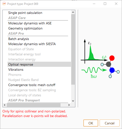
Fig. 6 Select Optical response from the project list.

Click on the Parameters icon to open the Optical response parameters widget.

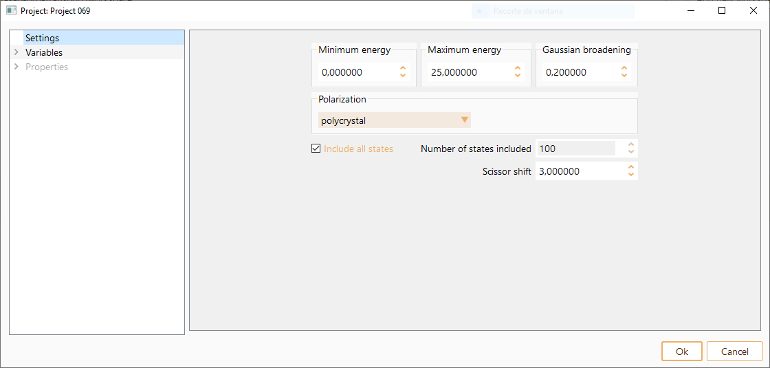
You can tune the following parameters:

• Minimum energy: Specifies the minimum value of the energy range (eV) in which the optical spectrum will be calculated.

• Maximum energy: Specifies the maximum value of the energy range (eV) in which the optical spectrum will be calculated. Please note that it is important to provide a large enough maximum energy.

• Gaussian broadening: The specified Gaussian broadening is applied to the optical spectrum.

• Polarization: ASAP offers the following three options:

  • polarized: The electric field is applied in a given direction. The direction of the applied electric field must be specified.

  • unpolarized: The light is propagated in a given direction. The direction of the light propagation must be specified. The different directions of the electric field within the perpendicular plane are averaged.

  • polycrystal (Default value): All possible directions of applied electric field and light propagation are averaged.

• Include all states: If checked all states are included in the optical property calculation.

• number of states included: Available only if Include all states is unchecked. It controls the number of states that are included in the optical property calculation. This number must be larger than the number of occupied bands and less than or equal to the number of basis functions (which determines the number of unoccupied bands available). Note that while including all the bands may be the most accurate choice this will also be the most expensive.

• Scissor shift: This number defines the rigid shift of the unoccupied states to be added to correct the gap and thereby improve the calculated results. The shift is only applied to the optical calculation and no where else within the calculation.

Click on the SIESTA_4.1 (calculator) icon to select SIESTA input parameters. Notice that the Optical response project is only available for the SIESTA calculator as warned in the project list, Fig. 6.

We refer the user to chapter Calculators for further information on the options offered by the SIESTA calculator widget.

Click on the Run icon to open the Run widget. Then press the Run button to submit the optical calculation.

We refer the user to chapter Runners for further information on computational resources configuration in ASAP.

While the calculation is running the Run widget shows the calculation output in real time.

Optical analysis

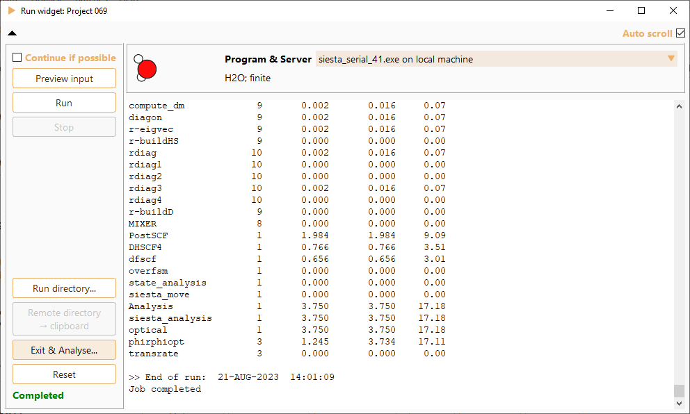
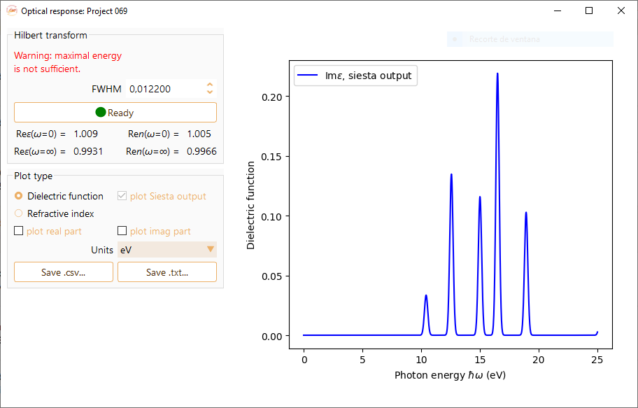
When the calculation is completed, select Exit & Analyse… to open the analysis widget.

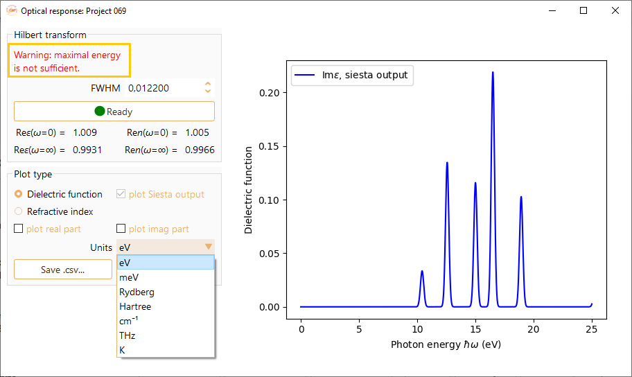
The analysis widget displays by default the imaginary part of the dielectric function computed directly from SIESTA. Frequency (energy) and Intensity of the absorption spectrum are shown on the x- and y-axis, respectively.

It is also possible to calculate the Hilbert transform to obtain the imaginary part of the dielectric function as well as the refractive index.

Note that a large enough energy range is necessary for the Hilbert transform, as the warning in the top left of the tab states. Additionally, you can tune the energy units, optionally eV, meV, Ry, Ha, cm ^-1, THz and K.

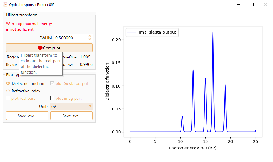
Tune the FWHM value and afterward click the Compute button to obtain the Hilbert transform.

Once you compute the Hilbert transform you can plot the dielectric functions as well as the refractive index.

You can plot the real and imaginary part of the dielectric function using the checkboxes plot real part and plot imag part, respectively.

For the dielectric function it is also possible to check the plot Siesta output check box to plot the original imaginary part of the dielectric function obtained directly from SIESTA.

Click the Refractive index option in Plot type to visualise the refractive index.

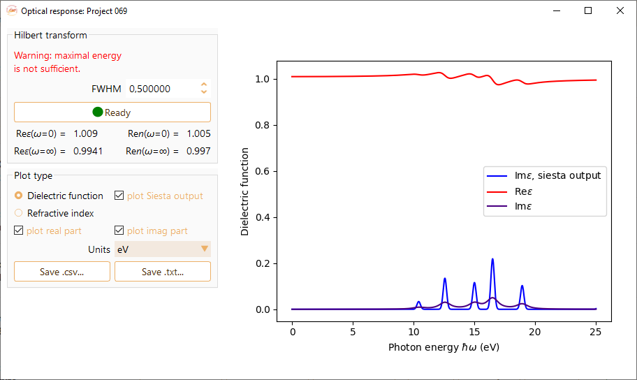
You can decide to visualize the real part and the imaginary using the check boxes plot real part and plot imag part, respectively.

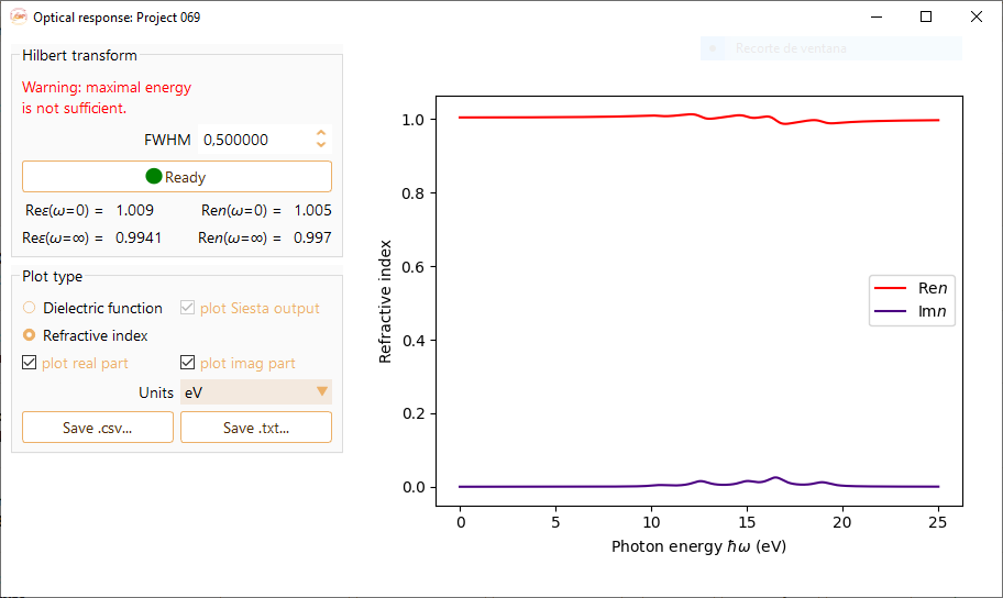
The quantities displayed right below the Compute button correspond to the real parts of the dielectric function (Re \(\varepsilon\)) and the refractive index (Ren) for limit values of the frequency.

Click the Save .csv… or the Save .txt… button to export the data in the preferred format.