Geometry Optimization

Geometry optimization determines the equilibrium structure of molecules and solids. The Geometry Optimization projects implemented in ASAP find the atomic arrangement corresponding to a local minimum of the energy.

A Geometry Optimization project starts with the definition of the atomic structure. We refer the user to section Structure Modeling in ASAP for further information on ASAP structure builder/viewer interface.

After the atomic structure is defined, edit the type of project.

Select one of the following options from the project menu:

• Geometry optimization (SIESTA Only): Compatible exclusively with the SIESTA calculator.

• Geometry Optimization (multicode): Works with all available calculators (EMT, SIESTA, Quantum ESPRESSO, and MACE).

With the EMT, Quantum ESPRESSO or MACE calculators, Geometry optimization (multicode) is the only option. With SIESTA both are available, and the choice depends on what your calculation requires:

• Geometry optimization (SIESTA only) reuses the wavefunctions and density matrix from the previous step as the starting point for the next one, which reduces the cost per step. Additionally, it avoids reinitializing the system infrastructure at each step, further speeding up simulation runs.

• Geometry optimization (multicode) gives access to the full set of ASE optimization algorithms and to a wider range of cell optimization modes.

Recommendation: If you are using the SIESTA calculator, select Geometry optimization (SIESTA Only) for optimal performance and faster calculations.

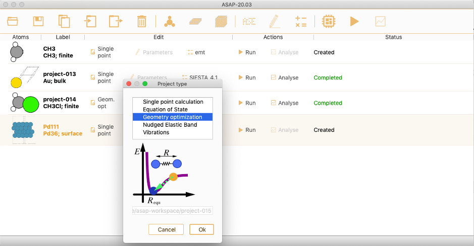
Then click on the Parameters icon to open the Geometry Optimization parameters widget.

Geometry optimization (SIESTA Only)

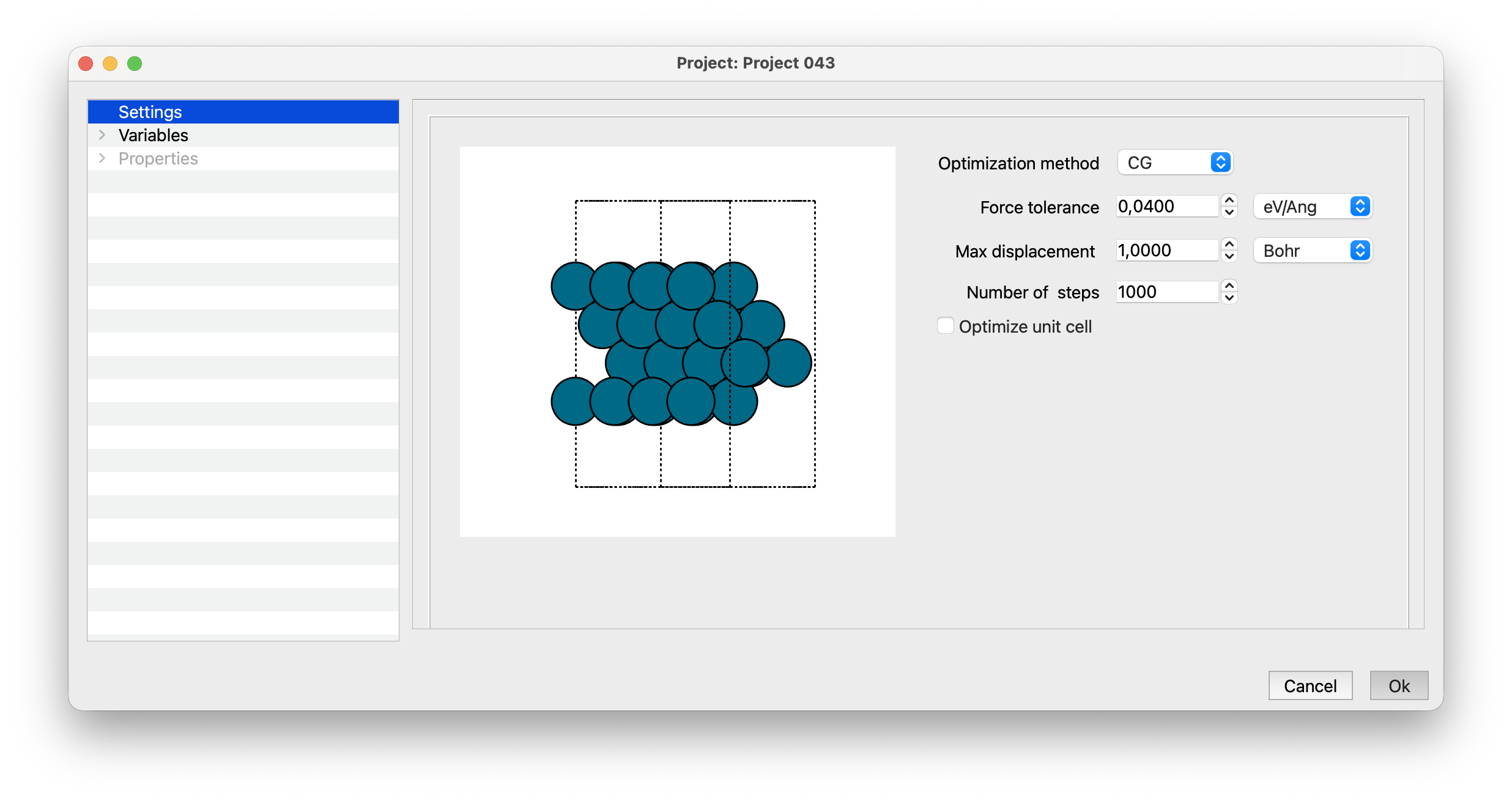
• Optimization method: SIESTA supports three methods: CG, Broyden and FIRE.

All methods share the following general parameters:

• Force tolerance: Specifies the convergence criterion. The simulation converges when the force on every individual atom is less than this value. In units of eV/Ångström, Ry/Bohr or meV/Ångström.

• Max displacement: Maximum allowed atomic displacement in a single optimization step. In units of Ångström, Bohr or nm.

• Number of steps: The maximum number of optimization steps allowed. If forces do not drop below the specified Force tolerance within these steps, the simulation will terminate without reaching full convergence.

• Optimized cell: Check the Optimize unit cell checkbox to allow cell relaxation alongside atomic positions, see section Optimize unit cell.

Optimize unit cell

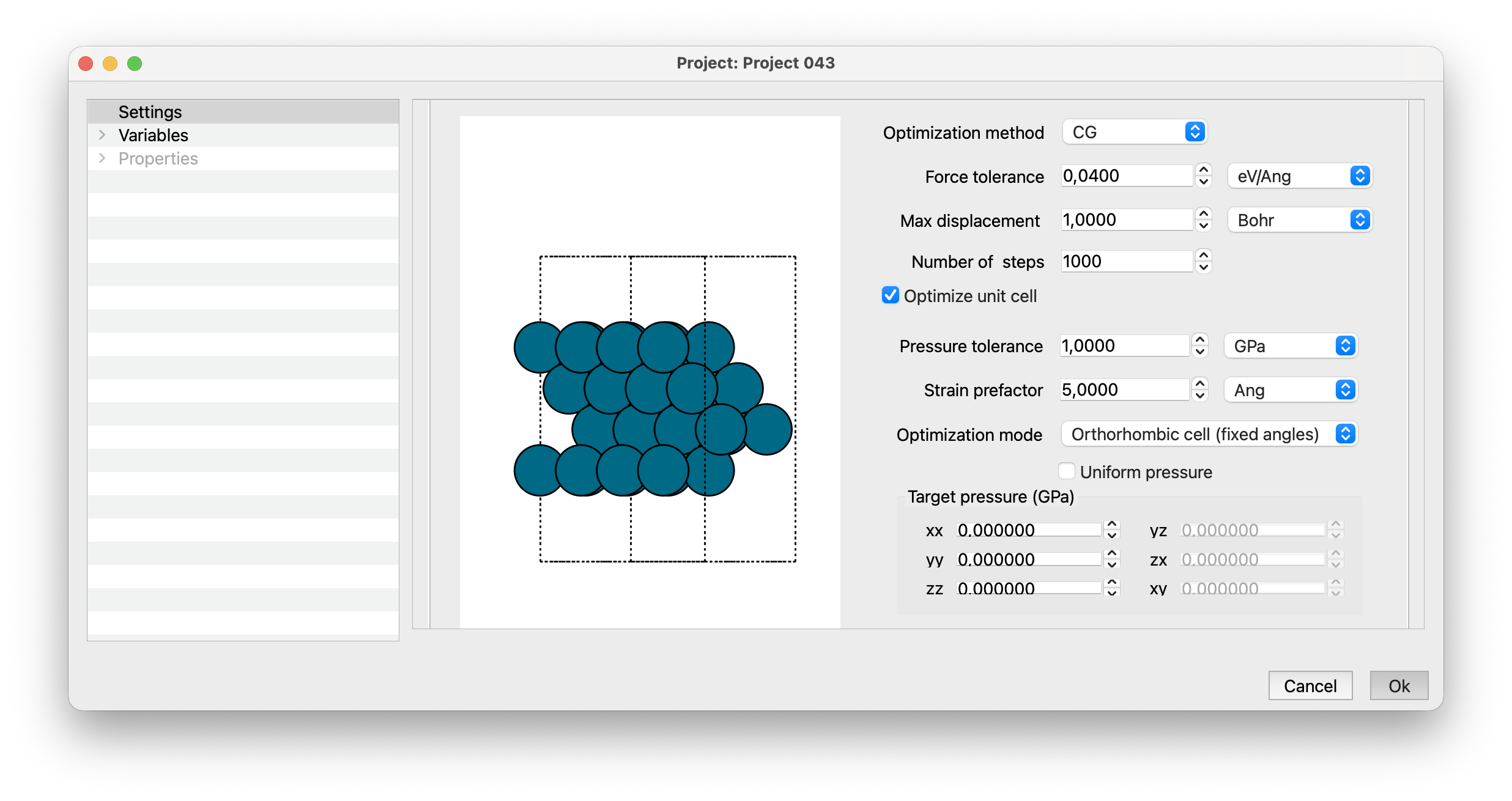
Checking the Optimize unit cell checkbox allows cell relaxation alongside atomic positions. This reveals additional cell-related parameters:

• Relax cell only: (Available only for Broyden or FIRE methods) If checked, it relaxes cell dimensions while rescaling atomic positions, maintaining constant fractional coordinates. If your system does not have a cell defined, a warning will pop up when you check this box. Click Yes to continue with the default unit cell, or define one in the 3D structure editor.

• Pressure tolerance: The convergence criterion for cell relaxation. The simulation completes successfully when both the maximum atomic force is lower than Force tolerance and the maximum stress tensor component is smaller than Pressure tolerance.

• Strain prefactor: Scales cell strain variations relative to atomic shifts during relaxation. Because atomic positions (Ångström) and dimensionless cell strains operate on different scales, this parameter multiplies the strains by the strain prefactor (Ångström) to ensure balanced, smooth convergence.

• Optimization mode: Select one of three available cell modes depending on the system’s structural constraints.

Orthorhombic cell (fixed angles)

When selected the following parameters will appear,

• Uniform pressure: Check this box to apply equal isotropic pressure across all directions. Uncheck it to specify independent pressure components.

• Target pressure (eV/Ang^3):

  • When the Uniform pressure is checked: A single value sets all diagonal target stress tensor components equally. Off-diagonal components are ignored during relaxation. The units correspond to the pressure unit selected in this widget.

  • When the Uniform pressure is unchecked: You can independently adjust each diagonal term (\(xx\), \(yy\), and \(zz\)) target stress tensor. The units correspond to the pressure unit selected in this widget.

Triclinic cell (fully flexible)

When selected the following parameters will appear,

• Uniform pressure: Check this box to apply equal isotropic pressure across all directions. Uncheck it to specify independent pressure components.

• Target pressure (eV/Ang^3):

  • When the Uniform pressure is checked: A single pressure value applies to all diagonal tensor components. Non-diagonal components are not considered during relaxation. The units correspond to the pressure unit selected in this widget.

  • When the Uniform pressure is unchecked: You can independently set every diagonal (\(xx\), \(yy\), and \(zz\)) and non-diagonal (\(yz\), \(zx\), and \(xy\)) term of the target pressure tensor. The units correspond to the pressure unit selected in this widget.

Constant volume

When selected the following parameters will appear,

• Uniform pressure: Check this box to apply equal isotropic pressure across all directions. Uncheck it to specify independent pressure components.

• Target pressure (eV/Ang^3):

  • When the Uniform pressure is checked: The stress tensor cannot be modified; target pressure is set to 0 for all tensor components. The units correspond to the pressure unit selected in this widget.

  • When the Uniform pressure is unchecked: You can independently adjust each diagonal and non-diagonal component of the target pressure tensor.

Geometry optimization (multicode)

Geometry Optimization (multicode) gives access to the full set of ASE optimization algorithms and to a wider range of cell optimization modes: Hydrostatic pressure and Hydrostatic pressure for selected axes are available only in this driver.

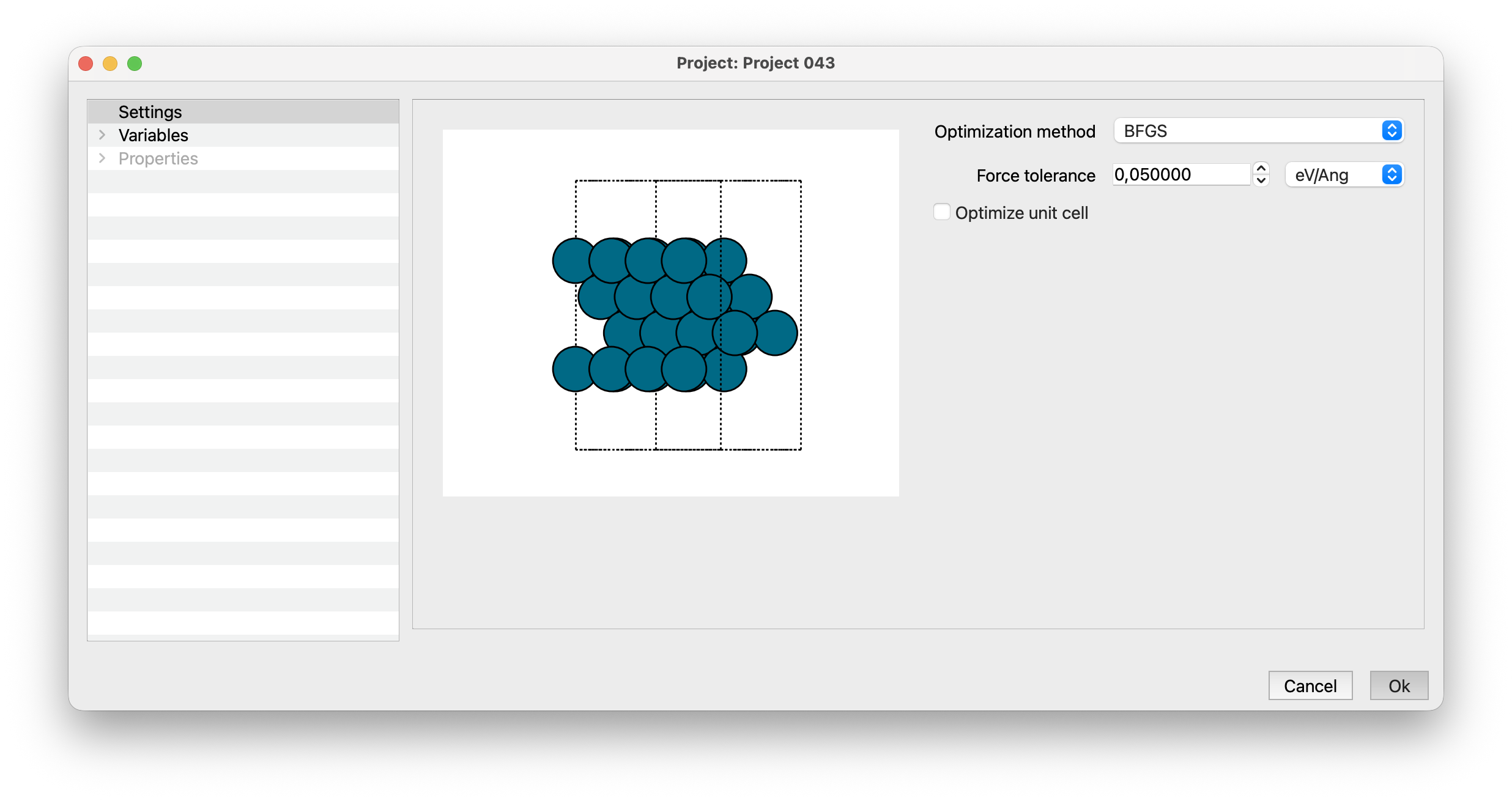
• Optimization method ASAP can make use of all the local Optimization algorithms available in ASE (https://docs.ase-lib.org/ase/optimize.html): BFGS, BFGSLineSearch, CellAwareBFGS, FIRE, FIRE2, GPMin, GoodOldQuasiNewton, LBFGS, LBFGSLineSearch, MDMin and ODE12r.

All the methods share the same parameters:

• Force tolerance: Specifies the convergence criterion. The simulation converges when the force on every individual atom is less than this value. In units of eV/Ångström, Ry/Bohr or meV/Ångström.

• Optimized cell: Check the Optimize unit cell checkbox to allow cell relaxation alongside atomic positions, see section Optimize unit cell for more details.

Optimize unit cell

Checking the Optimize unit cell checkbox allows cell relaxation alongside atomic positions. This reveals additional cell-related parameters that are common to all the Optimization methods.

If your system does not have a cell defined, a warning will pop up when you check this box. Click Yes to continue with the default unit cell, or define one in the 3D structure editor.

• Relax cell only:

  • If checked, it relaxes cell dimensions while rescaling atomic positions, maintaining constant fractional coordinates. You can select which stress tensor components to relax during the optimization process: xx, yy, zz, yz, zx, xy. Optimization mode and Target pressure are disabled.

  • If unchecked it allows setting the Optimization mode choosing from:

    • Hydrostatic pressure

    • Hydrostatic pressure for selected axes

    • Orthorhombic cell (fixed angles)

    • Triclinic cell (fully flexible)

    • Constant volume

• Optimization mode: determines which components of the stress tensor are relaxed. Five modes are available: Hydrostatic pressure, Hydrostatic pressure for selected axes, Orthorhombic cell (fixed angles), Triclinic cell (fully flexible) and Constant volume. See Target pressure below for what each mode controls.

Target pressure

The target pressure sets the value that the active components of the stress tensor are driven toward during the relaxation. Which components are active is determined by the Optimization mode: a single target value applies to all of them, expressed in the units selected in this widget. Components that are not active are ignored during the relaxation and are left unconstrained.

• Hydrostatic pressure: All three diagonal components are active and constrained to be equal. Off-diagonal components are ignored.

• Hydrostatic pressure for selected axes: Only the diagonal components you select are active. Off-diagonal components are ignored. Hydrostatic pressure means applying an isotropic stress tensor, which requires the diagonal components \(xx\), \(yy\), and \(zz\) to be equal, causing the corresponding cell axes to scale together by the same factor.

• Orthorhombic cell (fixed angles): Only the diagonal components you select are active, so the cell angles remain fixed. Off-diagonal components are ignored.

• Triclinic cell (fully flexible): Both diagonal and off-diagonal components can be selected, allowing the cell angles to change.

• Constant volume: The target pressure is fixed at zero for all components and cannot be edited; you select which components are relaxed.

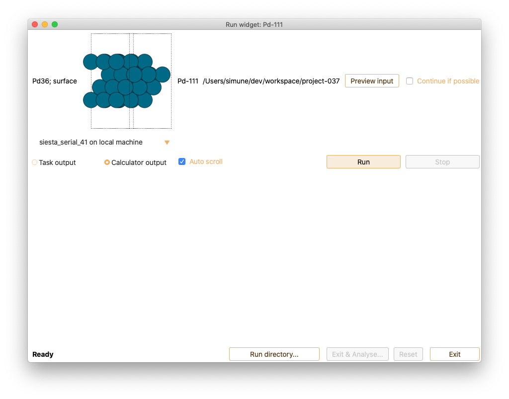
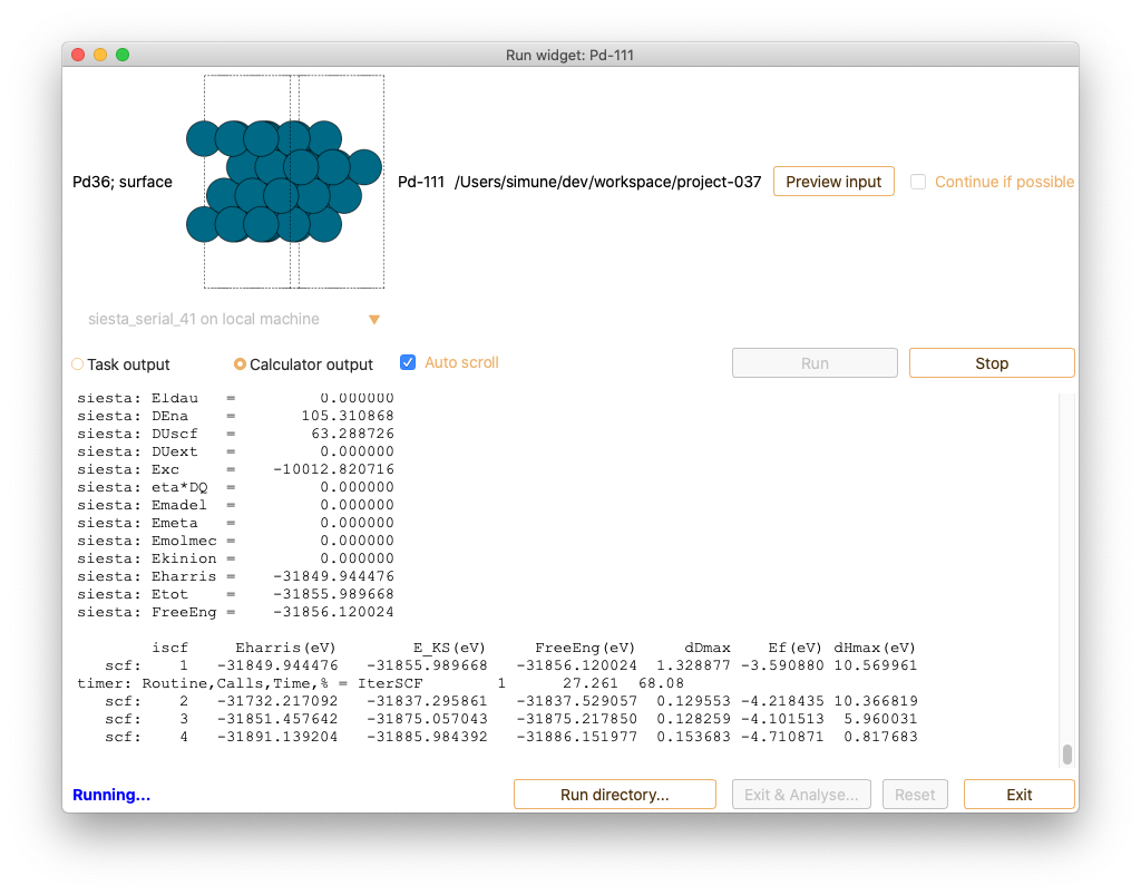
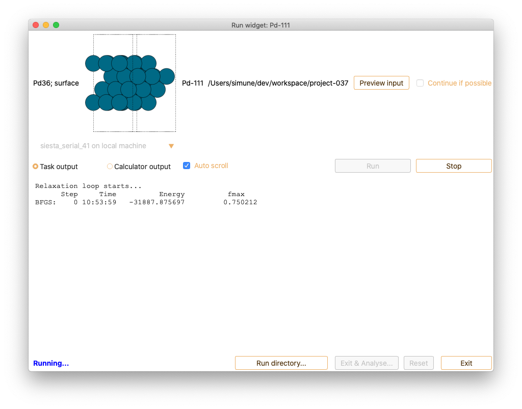
Select the calculator and run GO

Click on the Calculator icon to select the computational engine to be used during geometry optimization.

We refer the user to chapter Calculators for further information on ASAP available calculators.

Click on the Run icon to open the Run widget. Then click on the Run button to submit the geometry optimization calculation.

We refer the user to chapter Advanced Configuration and Remote Execution for further information on computational resources configuration in ASAP.

After submitting a job (run), the tab Calculator output in the Run widget shows the complete calculation output in real time.

In addition, if you are running a Geometry optimization (multicode) project, you can monitor the geometry optimization steps and corresponding system total energy in real time using the Task output tab.

Analysis

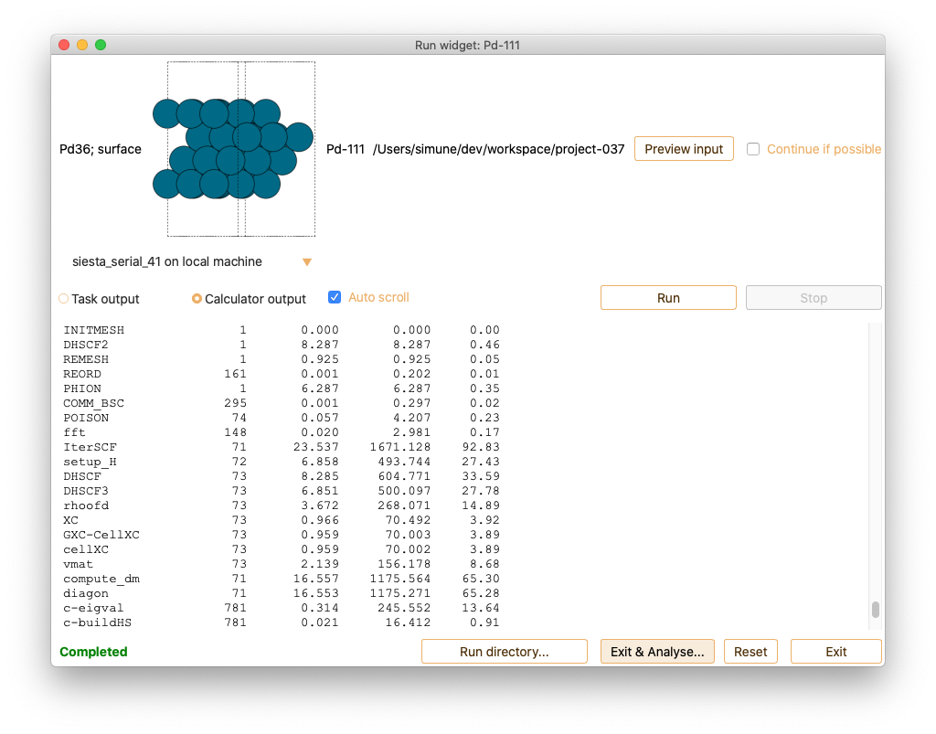
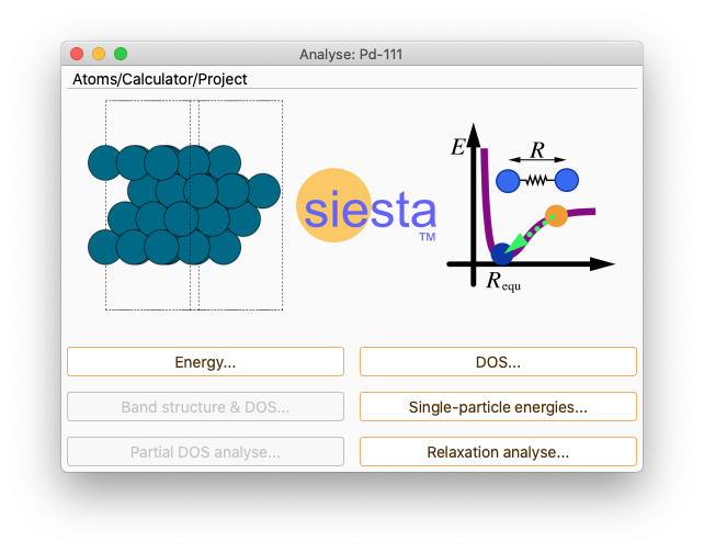
When the calculation is completed, select Exit and analyse to open the analysis widget.

The analysis widget plots the total energy of the system against the optimization step, so you can check how the relaxation converged. The atomic structure corresponding to the selected step is shown in the right panel.

From the analysis widget you can:

• Current image: Change the selected step (image) to display as a point on the chart and as an atomic structure on the right panel.

• View angles: Change the structure viewing angles.

• Wrap to the box: In some cases the structure might extend outside the box; check this checkbox if you want to visualize the structure entirely inside the unit cell box.

• View in 3D…: Visualize the evolution of the atomic structure at each step of the geometry optimization.

• Export current image…: Save the currently viewed structure image on your machine in various formats.

• New project: Start a new project using the computed optimized structure.

• Copy to clipboard: Copy the total energy (in eV) of the relaxed structure to your clipboard.