Calculators#
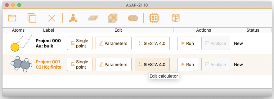
ASAP implements the EMT calculator, the SIESTA and TranSIESTA calculators and the Quantum ESPRESSO calculator.
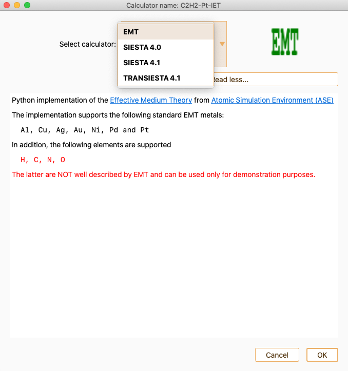
The EMT Calculator#
ASAP incorporates the Effective Medium Theory (EMT) calculator as implemented in Atomic Simulation Environment (ASE). EMT

The SIESTA Calculator#

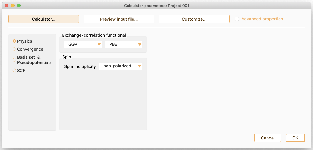
You can specify key input variables through the SIESTA calculator graphical user interface.
ASAP classifies SIESTA parameters in the following categories:
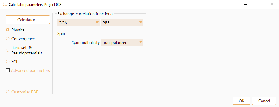
Physics: It aggregates parameters related with exchange correlation functional and spin. See SIESTA Parameters: Physics.
Convergence: Real-space mesh cutoff energy and Brillouin Zone Sampling. See SIESTA Parameters: Convergence.
Basis set and Pseudopotentials. See SIESTA Parameters: Basis set and Pseudopotentials.
SCF. It aggregates parameters controlling Self Consistent Field (SCF) convergence. See SIESTA Parameters: SCF.
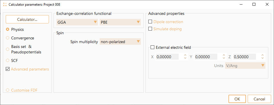
Click the Advanced properties button to enable advanced input parameter widget for all categories.
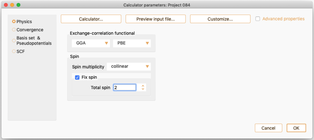
The SIESTA calculator also allows to preview and edit the SIESTA input file, see sections Preview input file and customise.
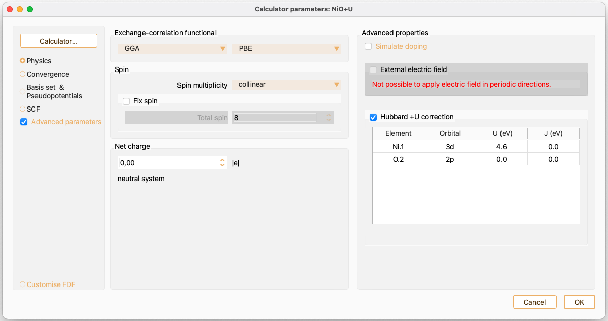
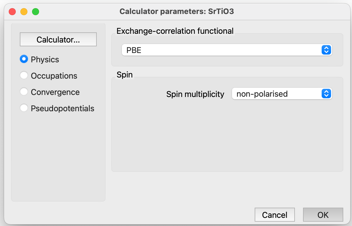
SIESTA Parameters: Physics#
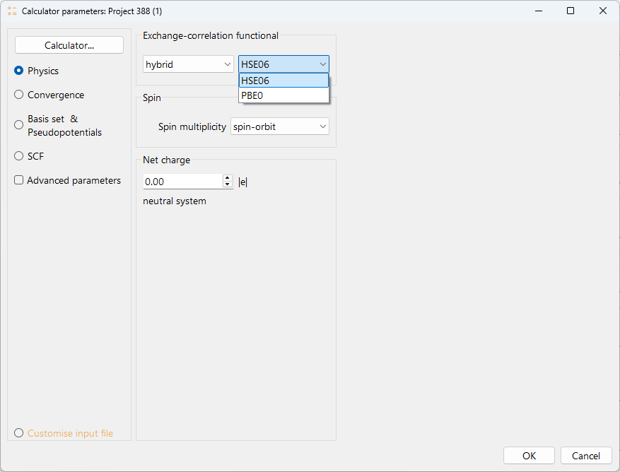
You can select one of the offered functional to specify the exchange-correlation functional type. The available options are:
LDA (Local Density Approximation)
GGA (Generalised Gradient Approximation)
VDW (Van der Waals)
hybrid* (Hybrid functionals)


collinear. To perform a calculation with collinear spin (two spin components).
non-collinear. To perform a calculation with non-collinear spin (four spin components), up-down and angles.
spin-orbit. To perform a calculation with spin-orbit coupling. This type of calculation requires the pseudopotentials to be relativistic.

Dipole correction (Advanced properties)#

Simulate doping (Advanced properties)#

External electric field (Advanced properties)#


Implicit solvent (Advanced properties)#
Implicit Solvation Environment: It models the solvent as a continuous dielectric medium, allowing for simulations of systems in a liquid environment while avoiding the high cost of explicit molecules. Note that the implicit solvent model adds computational complexity: for molecules, expect an increase in SCF step time by roughly an order of magnitude, whereas for large slab systems, the overhead is significantly lower, typically a factor of ~1.5.
Exact Boundary Condition Treatment: It allows for the determination of the electrostatic potential under various conditions (bulk, surface, wire, and free). This effectively enables SIESTA to function as a non-periodic or semi-periodic code, eliminating spurious long-range interactions between periodic images in isolated or slab systems.
Core Features
Generalized Poisson Equation (GPe) Solver: Interfaces SIESTA with the PSOLVER library from the BigDFT suite to solve the GPe exactly under arbitrary boundary conditions.
Soft-Sphere Cavity: The dielectric cavity is constructed from atom-centered, interlocking smooth spheres. The transition from vacuum (\(\epsilon=1\)) to the bulk solvent permittivity (\(\epsilon_s\)) is handled by a smooth function that prevents numerical instabilities during force calculations.
Non-Electrostatic Terms: The model accounts for cavitation, repulsion, and dispersion energy contributions by using a linear combination of the solute’s quantum surface (\(S^{cav}\)) and quantum volume (\(V^{cav}\)).
It supports orthorhombic cells, but not cell with angles \(\ne 90^\circ\).
It does not compute the stress tensor, as it has no physical relevance in the context of implicit solvent.
The PSML format for pseudopotentials is incompatible with psolver. Therefore, the use of PSF pseudopotentials is required. In ASAP, the appropriate pseudopotential is automatically selected when the user chooses the implicit solvent option.
Physical Approximations of the Model
The exchange-correlation contribution arising from the overlap between solute and solvent electron densities is neglected.
The core electrons of the solute are considered frozen and unaffected by the dielectric function (the non-local part of the pseudopotential is unchanged). The overlap of ionic charge densities is approximated as if the system were in a vacuum.
Self-interaction energies are calculated as in a vacuum, which introduces a slight energy shift for a given geometry.
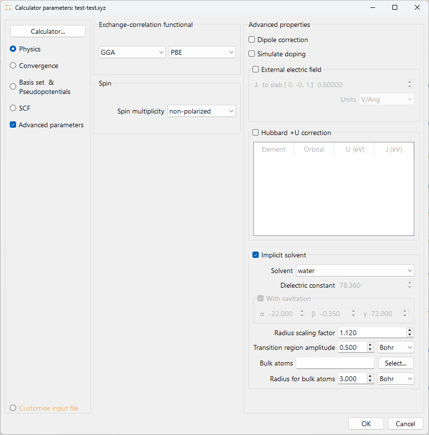
Fig. 29 Calculator widget advanced parameters, implicit solvent.#
Parameter Configuration
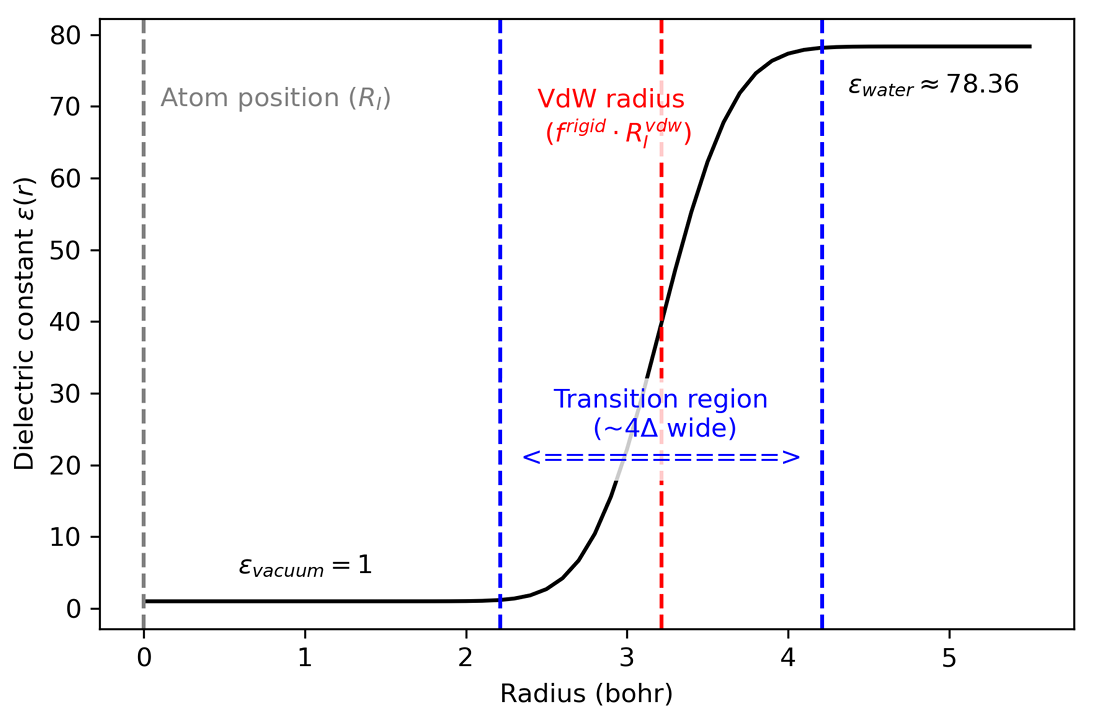
Fig. 30 Radial shape of the dielectric function centered on an isolated atom.#
Solvent: Selects the solvent model from the dropdown list. This choice sets the default values for the options below.
Water: Automatically sets the Dielectric constant to the standard value for water (e.g., 78.360) and checks the With cavitation box by default.
Custom: Enables the Dielectric constant field for manual input and leaves the With cavitation box unchecked by default.
Dielectric constant (:math:`epsilon`): Defines the dielectric constant of the continuum solvent. This field is automatically populated when water (78.36) is selected and is manually editable when custom is chosen. Setting epsilon to 1.00 is equivalent to vacuum calculation.
With cavitation: Check this box to include the corrective non-electrostatic term. This box is checked by default for water and unchecked by default for custom, but can be toggled manually in the latter case. When custom is selected and the With cavitation box is checked, the following coefficients must be specified:
\(\alpha\): Proportionality of the short-range Pauli exchange repulsion free energy in terms of the quantum surface of the solute cavity [dyn/cm]. Default value -22.
\(\beta\): Proportionality of the van der Waals dispersion free energy in terms of the quantum volume of the solute cavity [GPa]. Default value -0.35.
\(\gamma\): Solvent surface tension, used to compute the cavitation energy (the energy required to separate solvent molecules to accommodate the solute) in terms of the quantum surface of the solute [dyn/cm]. Default value 72.
Radius scaling factor (:math:`f^{rigid}`): A dimensionless factor used to scale the atomic VdW radii (\(R_I^{VdW}\)) that defines the boundary of the rigid cavity. The sphere radius (\(R^I_{sphere}\)) is defined as (\(R^I_{sphere} = f_{rigid} × R_I^{VdW}\)). Using 1.00 means that we use (\(R_I^{VdW}\)) directly as (\(R_I^{sphere}\)). Default value 1.120.
Transition region amplitude (:math:`Delta`): Defines the width of the dielectric transition between the solute and the solvent. You can specify the units in the adjacent dropdown menu. Default value 0.500 Bohr. A very small value causes numerical inaccuracies, as the dielectric function becomes too sharp for the real-space discretization. On the other hand, a very large value for \(\Delta\) leads to a non-physical approximation, as it overestimates solvent penetration into the system.
Bulk atoms: This field identifies atoms that are part of a bulk material (part of a surface or slab) and should not be exposed to the solvent. You can specify these atoms in two ways:
Manual Input: Type the atomic indices directly into the text field (e.g., 1, 2, 5-10).
Graphical Selection: Click the Select… button to open the atomic structure viewer. Within the viewer, select the atoms you want to define as “bulk” (e.g., by using the “fix atoms” tool). Once fixed, atom indices will be automatically added to the Bulk atoms field.
Radius for bulk atoms (:math:`R_{bulk}`): Defines a sphere radius \(R^I_{sphere}\) for the selected Bulk atoms to ensure the interior of the material remains excluded from solvent effects. You can specify the units in the adjacent dropdown menu. Default value 3.000 Bohr.
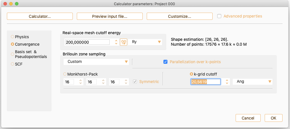
SIESTA Parameters: Convergence#
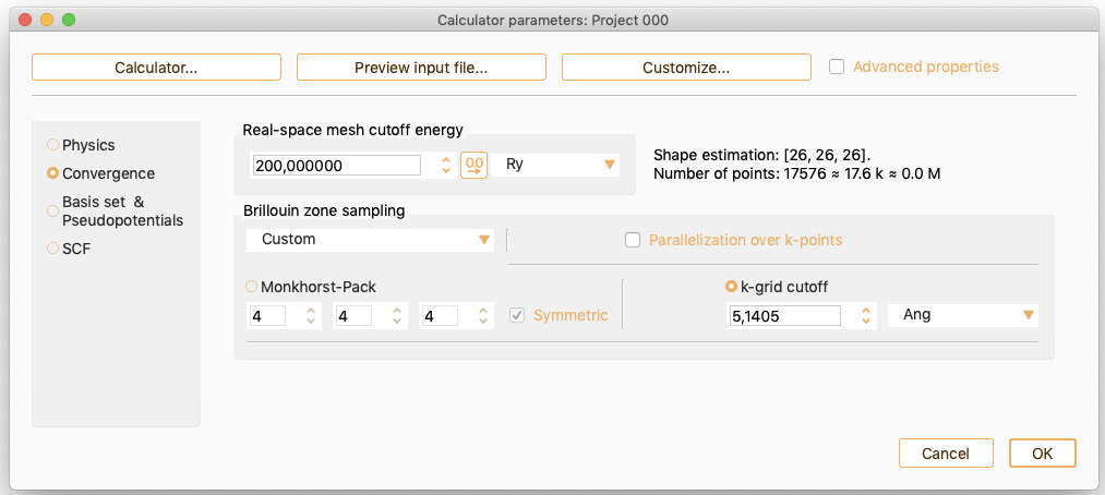


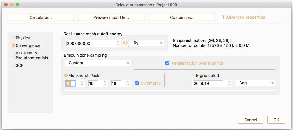
As an alternative, click the k-grid cutoff button to specify the parameter which determines the fineness of the k-grid used for Brillouin zone sampling.
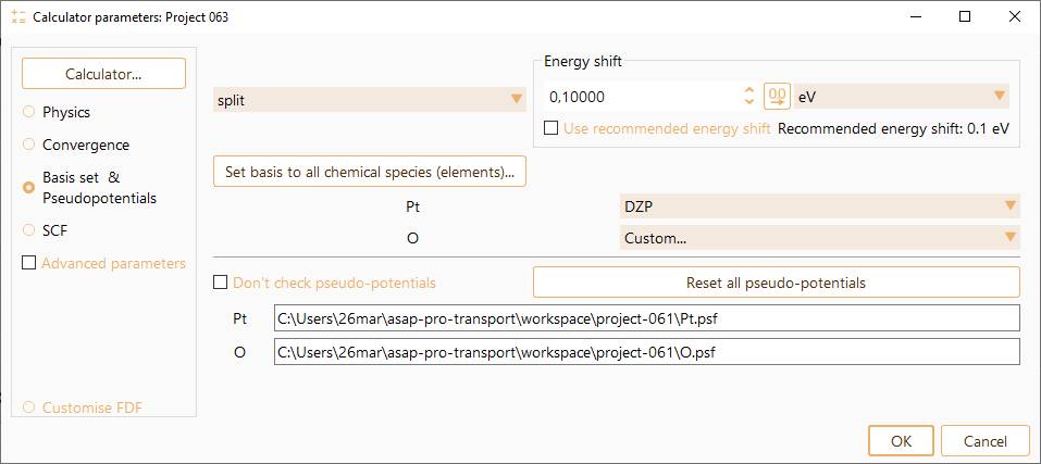
SIESTA Parameters: Basis set and Pseudopotentials#

Basis set
SIESTA code makes use of local atomic orbital basis set to describe the valence electrons. SIESTA generates extended bases by applying the Split-valence scheme for multiple-zeta. The split is based on different radii. The user has the possibility to choose among the different options available for basis generation and basis size.
First, the kind of basis to be generated is chosen. All are based on finite-range pseudo-atomic orbitals. PAO’s of Sankey and Niklewsky, PRB 40, 3979 (1989).

Basis size
This parameters indicates the number of orbitals per atom.
SZ or MINIMAL: Minimal or single-zeta basis set (no polarisation).
DZ: Double zeta basis set (without polarisation functions).
SZP: Single-zeta basis plus polarisation orbitals.
DZP: Like DZ plus one polarisation orbital. Polarisation orbitals are constructed from perturbation theory, and they are defined so they have the minimum angular momentum \(l\) such that there are not occupied orbitals with the same \(l\) in the valence shell of the ground-state atomic configuration. They polarise the corresponding \(l\)-1 shell.
DZP2: Double zeta basis plus two polarisation orbitals.
TZ: Triple zeta basis set.
TZP: Triple zeta basis plus one polarisation orbital.
TZP2: Triple zeta basis plus two polarisation orbitals.
TZP3: Triple zeta basis plus three polarisation orbitals.

A more complete basis set (higher number of basis functions) allows, in principle, more accurate simulations. However, per se, the total number of basis functions does not guarantee more accuracy, other basis set parameters such as Energyshit and the Basistype are fundamental to get good accuracy.
It is possible to set the same basis size for all chemical species present,
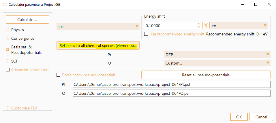
and also to use different basis size for each of the elements.

Pseudopotentials

SIESTA Parameters: SCF#
SIESTA uses the standard Kohn-Sham self-consistent Density Functional Method (DFT). SCF widget aggregates parameters controlling SCF converge.

Maximal number of iterations.
Hamiltonian. Mix the Hamiltonian matrix.
Density. Mix the density matrix.
Charge. Mix the real-space charge density. Note this is an experimental feature in SIESTA.
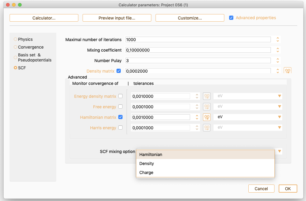
The advanced parameters widget offers the following additional options to control SCF convergence:
Energy density matrix. Option only available since Siesta version 4.1. Click on this check box to make use of the energy density matrix elements as monitor of self-consistency. The self-consistency is considered achieved when the maximum absolute change (dEmax) in the energy density matrix elements is below the specified tolerance value.
Free energy. Click on this check box to make use of the change in the total (free) energy between cycles of the SCF procedure as a monitor of self-consistency. The self-consistency is achieved when the change in the total free energy between cycles of the SCF procedure is below the specified tolerance value and the density matrix change criterion is also satisfied.
Hamiltonian matrix. Option only available since Siesta version 4.1. Click on this check box to make use of the Hamiltonian matrix elements as a monitor of self-consistency. The self-consistency is achieved when the maximum absolute change (dHmax) in the H matrix elements is below the specified tolerance value. The actual meaning of dHmax depends on the selected SCF mixing option:
if mixing the Density Matrix, dHmax refers to the change in H(in) with respect to the previous step.
if mixing the Hamiltonian matrix, dHmax refers to H(out)-H(in) in the previous step.
Harris SCF Convergence. Click on this check box to use the Harris energy as monitor of self-consistency. The self-consistency is achieved when the change in the Harris energy between cycles of the SCF procedure is below the specified tolerance value.
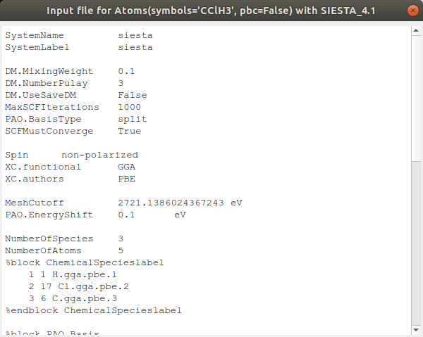
Preview input file#
The button Preview input file allows to view the created SIESTA .FDF input file with the GUI of the SIESTA calculator.
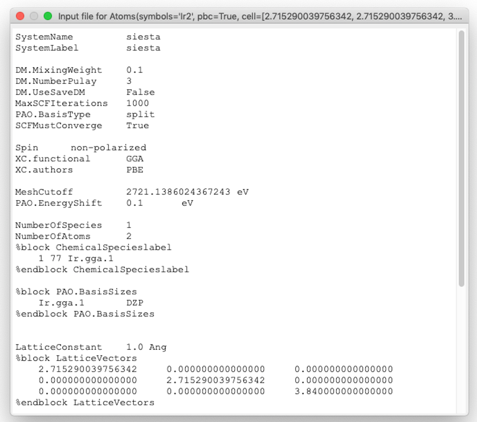
The .FDF file (Flexible Data Format) file, developed by A. Garcia and J.M. Soler includes physical data of the system as well as the variables to control the approximations used in the calculation. Whereas the former parameters are mandatory, others have default values assigned and, in principle, it is not necessary to explicitly include them in the input file. However, it is important to stress out that the default values do not always guarantee an accurate and converged calculation.
customise#

Get from widget. To rewrite the input file with the data from widgets (graphical user interface).
Save to update the calculator.
The TranSIESTA calculator#

The TranSIESTA code allows to solve the electronic structure of an open system formed by a finite structure sandwiched between two semi-infinite metallic leads. A finite bias can be applied between both leads, to drive a finite current.

You can specify key input variables through the TranSIESTA calculator graphical interface.
Additionally to the settings commonly used for the SIESTA calculations, see section The SIESTA Calculator, there are new tabs specifically designed for setting up the transport calculations. Click the Advanced properties button to enable advanced input parameter widget for all categories.
Device: To set up the parameters for the description of the Electrode and the Charge correction.
Integration contours (Advanced properties): Used to set up the details of the contour integration.

Density matrix update: It controls which part of the electrode density matrix elements are updated. Select one of the following options:
All (Default value): Both the density matrix elements in the electrode and the coupling elements between the electrode and scattering region. It provides most accurate results.
Cross-terms: To update only the coupling elements between the electrodes and the scattering region.
None: To update only the density matrix elements of the scattering region.
Green function imaginary part: It controls the imaginary energy of the surface Green function for this electrode. Ensure that all imaginary values are larger than 0 as otherwise TranSIESTA may seg-fault.
Impose bulk Hamiltonian: Control whether the Hamiltonian of the electrode region in the scattering region is enforced bulk or whether the Hamiltonian is taken from the scattering region elements. If Density matrix update is set to “all”, the “Impose bulk Hamiltonian” option is not enabled.
Charge correction
Charge correction: Any excess/deficiency of charge can be re-adjusted after each TranSIESTA cycle to reduce charge fluctuations in the cell. We recommend to only use charge corrections for 0 V calculations. ASAP offers the following options:
none: No charge corrections are introduced. Recommended for calculations with voltage applied.
buffer (default value): Excess/missing electrons are placed in the buffer regions.
fermi: Corrects the charge filling by calculating a new reference energy level.
Factor (Enabled only if Charge correction is set to buffer or fermi): This option helps to reduce the fluctuations in the SCF. Default value 0.75. Select a value between 0 (no charge correction) and 1 (total charge correction) If Charge correction is set to fermi), you can also tune the following parameters:
Tolerance (Enabled only if Charge correction is set to fermi): The tolerance at which the charge correction will converge. Any excess/missing charge (\(|Q_0-Q|>\mathrm{Tolerance}\)) will result in a correction for the Fermi level. Default value 0.01.
Max Fermi level shift (Enabled only if Charge correction is set to fermi): The maximum allowed value that the Fermi level will change from a charge correction using the Fermi correction method. If you know the band-gap, setting this to 1/4 (or smaller) of the band-gap seems like a better value than the rather arbitrarily default one. Default value 1.5 eV.
Eta for Fermi method (Enabled only if Charge correction is set to fermi): To select the value at which the charge at the poles are extrapolated. Usually a smaller value will imply larger changes in the Fermi level. We recommend to increase this value if the charge convergence with respect to the Fermi level suffers strong fluctuations. Default value 0.001 eV.
only for 0 V (Enabled only if Charge correction is set to fermi): Apply the charge correction only for 0 V calculation, by default the box is checked.

Electronic temperature: Define the temperature used for the Fermi distributions for the chemical potentials.
Equilibrium contours
Circle part: To define the equilibrium contours of the circle part. You can select one of the following options,
Minimal energy: Define the minimum energy in the x-axis for the integration. It should be lower than the lowest eigenvalue. Default -40 eV.
Number of points: Define the number of integration points for the circle part of the integration contour. Default 30.
Tail part: To define the equilibrium contours of the tail part, you can select one of the following options,
Imaginary energy: The imaginary part of the line integral crossing the chemical potential. Default enabled, value 2.5 eV.
Number of poles: Alternative to Imaginary energy. Manually select the number poles for the equilibrium contour.
Number of points: Define the number of integration points for the tail part of the contour. Default 10.
The user can also define the number of of integration points for the tail part of the contour (“Number of points”).
Bias contour
Integration step: Define the number of integration points/energy separation. Default value 0.01 eV.
Fermi function cutoff: The bias contour is limited by the Fermi function tails. Numerically it does not make sense to integrate to infinity. This energy defines where the bias integration window is turned into zero. Default value 5 kT.

The Quantum ESPRESSO Calculator#

ASAP categorised Quantum ESPRESSO parameters into the following groups:
Physics: This category includes parameters related to the exchange correlation functional and spin. For more details, refer to section Quantum ESPRESSO Parameters: Physics.
SCF: This category involves selecting the method used to determine how electrons are distributed within the electronic energy levels of the system. It also aggregates parameters controlling Self Consistent Field (SCF) convergence. For more details, refer to section Quantum ESPRESSO Parameters: SCF.
Convergence: Parameters in this category cover real-space mesh cutoff energy and Brillouin Zone Sampling. For additional information, see Quantum ESPRESSO Parameters: Convergence.
Pseudopotential. See Quantum ESPRESSO Parameters: Pseudopotentials.
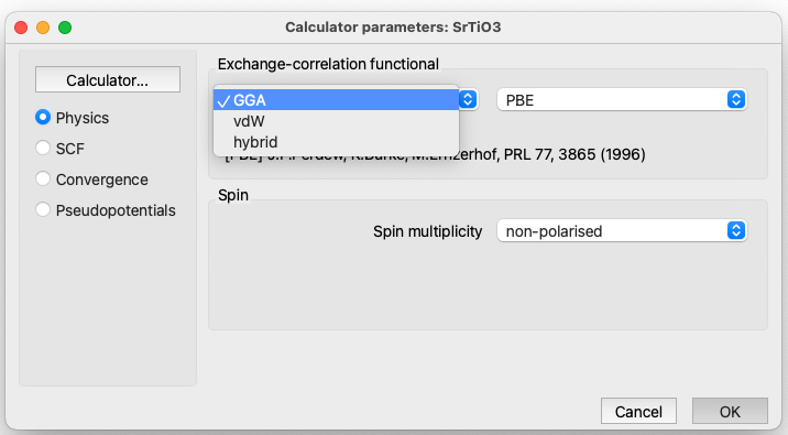
Quantum ESPRESSO Parameters: Physics#
LDA (Local Density Approximation)
GGA (Generalised Gradient Approximation)
hybrid (Hybrid functionals)

collinear. To perform a calculation with collinear spin (two spin components).
non-collinear. To perform a calculation with non-collinear spin (four spin components), up-down and angles.
spin-orbit. To perform a calculation with spin-orbit coupling. This type of calculation requires the pseudopotentials to be relativistic.
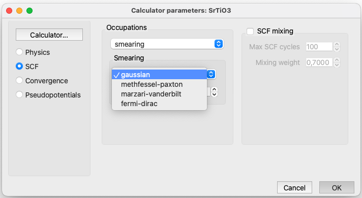
Quantum ESPRESSO Parameters: SCF#
This category involves selecting the method used to determine how electrons are distributed within the electronic energy levels of the system.

The options are:
smearing. Method using a smearing technique to distribute electrons over energy levels. You can also select the variable controlling the smearing. For the option Gaussian, you can select the value of the gaussian spreading (Ry) for brillouin-zone integration in metals.Gaussian smearing for metals.

tetrahedra. Tetrahedron method. P.E. Bloechl, PRB 49, 16223 (1994) Well suited for calculation of DOS.
tetrahedra-lin. Original linear tetrahedron method. To be used only as a reference. The optimised tetrahedron method is more efficient.
tetrahedra-opt. Optimised tetrahedron method. M. Kawamura, PRB 89, 094515 (2014). Can be used for phonon calculations as well.
fixed. For insulators with a gap
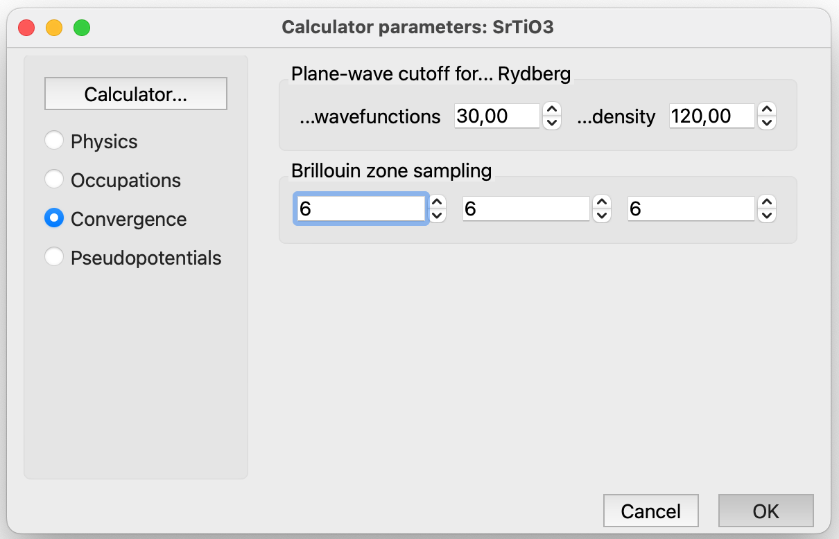
Quantum ESPRESSO Parameters: Convergence#
Plane wave cutoff for wavefunctions. This refers to the kinetic energy cutoff (in Rydbergs) used for wavefunctions.
Plane wave cutoff for density. This corresponds to the kinetic energy cutoff (in Rydbergs) for charge density and potential. For norm-conserving pseudopotential, it is advisable to set this value at least 4 times the kinetic energy cutoff used for wavefunctions. Reducing it too much may introduce noise, especially in forces and stress calculations. In the case of ultrasoft pseudopotentials, a larger value is often desirable, typically ranging from 8 to 12 times the kinetic energy cutoff used for wavefunctions.
Quantum ESPRESSO Parameters: Pseudopotentials#
