Local density of states (LDOS)

This type of project describes a space-resolved density of states. The LDOS project is useful in inhomogeneous systems. The LDOS project is useful to describe inhomogeneous systems. For instance, in a slab, the surface’s band structure differs from the bulk.. LDOS is also useful when interpreting the data from a scanning tunnelling micrope (STM), since this method is capable of imaging electron densities of states resolutions.

A LDOS project starts with a previously completed single-point project calculated with SIESTA calculator. We refer the user to section Single-point calculation for further information on single-points calculations.

After the single-point project has been calculated, select LDOS from the list of possible project types implemented in ASAP. We recommend creating a duplicate of the project, including the acquired results. Then, from the copied project, change the project type instead of changing it in the original one. This will keep the results from the single-point calculations intact.

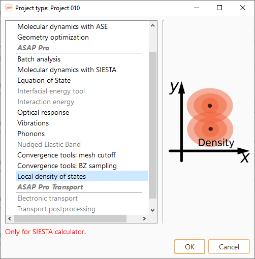
Then click on the Parameters icon to open the LDOS parameters widget.

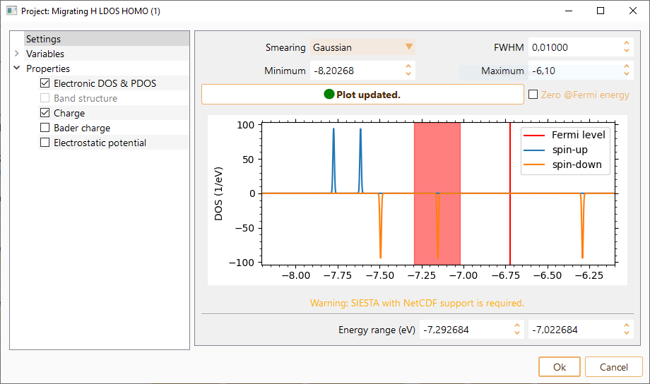
The widget will show the computed DOS from the previously completed calculation. It will help you to decide the relevant energy range for LDOS computation. You can tune the following parameters related to DOS visualisation:

• Smearing: Gaussian or Lorentzian representations of Dirac delta function.

• FWHM: The full width at half maximun. It is the distance used between the calculated points to perform the smearing. Click on the Zero at Fermi level check box to center DOS at the fermi level.

• Minimum: Minimum energy for DOS visualisation.

• Maximum: Maximum energy for DOS visualisation.

Press the OK button to save and close the Parameters widget.

The computation of LDOS requires using SIESTA version compiled with NetCDF library. We refer the user to chapter Calculators for further information on ASAP available calculators.

Click on the Run icon to open the Run widget.

We refer the user to chapter Runners for further information on computational resources configuration in ASAP.

Click on the Run button to execute the calculation.

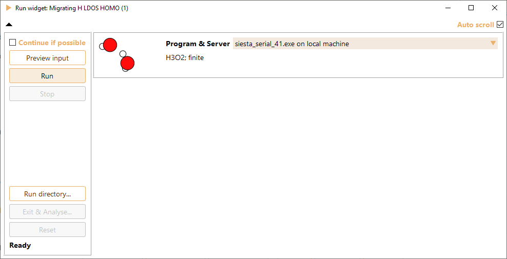
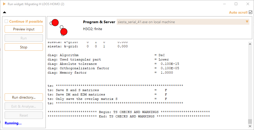
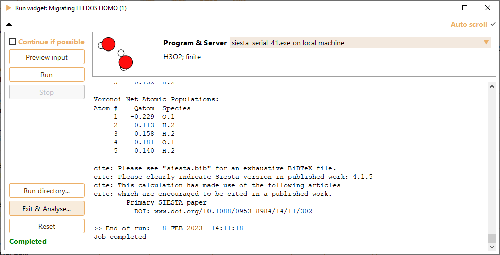
After submitting a job, the complete calculation output in real time is shown in the Run widget.

Analysis

When the calculation is completed, press the Exit and analyse button to open the LDOS analysis widget.

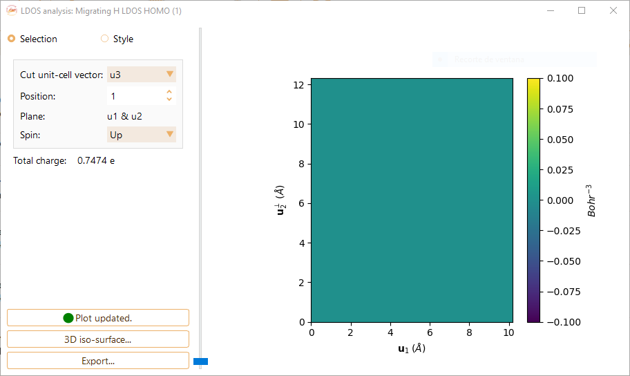
Click on the Selection button to tune the following parameters:

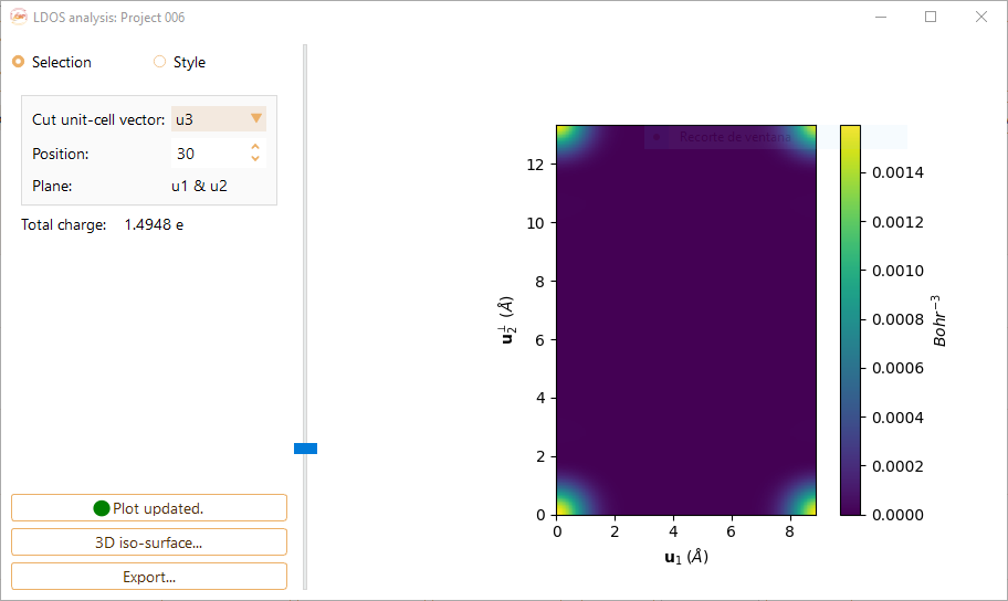
• Cut unit-cell vector.You can choose the cut unit-cell among the vectors u1, u2 and u3. It will defined the 2D plane for LDOS visualisation.

  

• Position.The position of the plot plane along the cut unit-cell vector. You can choose the desired index from the stored data.

  

• Spin.The options are Up + Down, Up and Down.

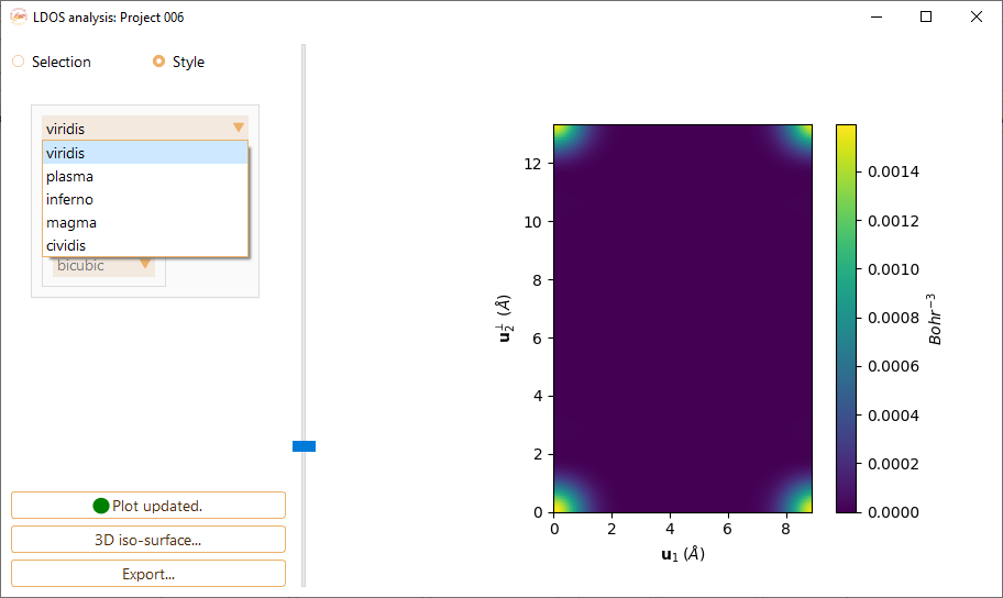
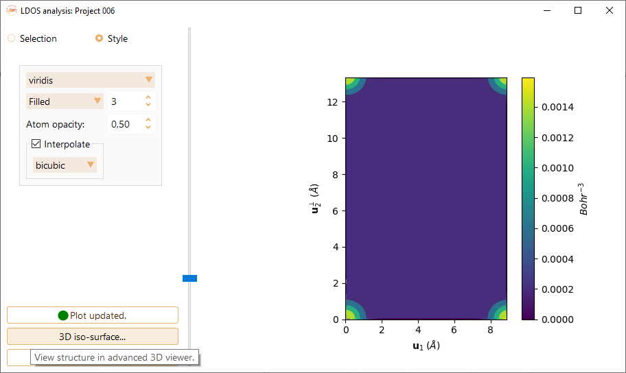
To change the style of the graphic click on the Style button. You can tune the following parameters:

• The color map.

  

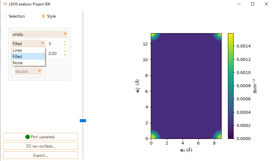
• The definition of the graphic.

  

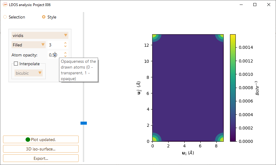
• Atom opacity.The opacity of the discs representing the atoms in the plot.

  

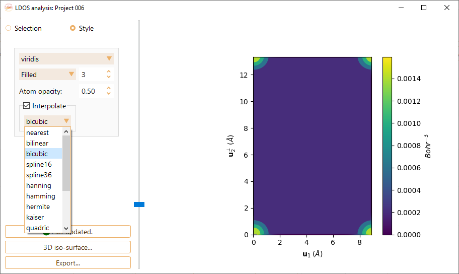
You have the option to click on the “Interpolate” button to perform data interpolation. ASAP offers the interpolation methods implemented in matplotlib.

Press the 3D iso-surface… button to view a three dimensional representation of the structure of the selected project.

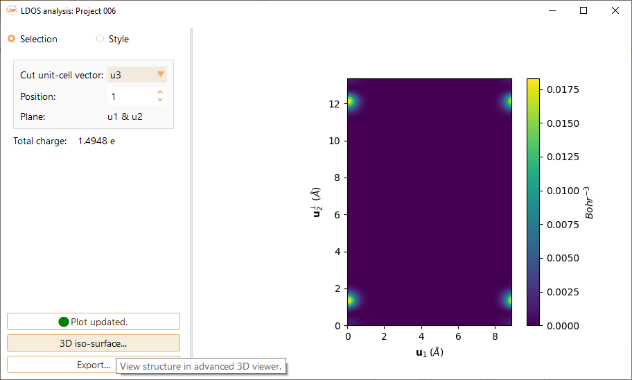
Press the Export… button to export the volumetric data of LDOS to .cube file. For spin polarised calculations, ASAP automatically exports three .cube files: up+down, up and down.

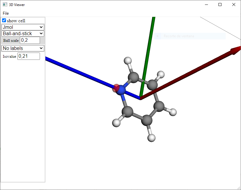
Advanced 3D viewer

Click the View in 3D button in the Analysis widget to obtain a three-dimensional representation of the structure of the material as well as a visualisation of the induced isopotential surface.

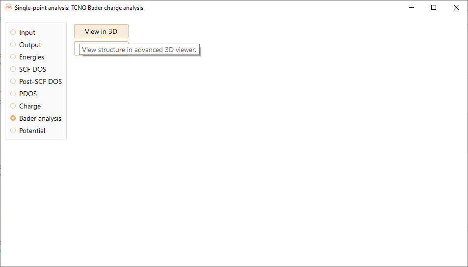
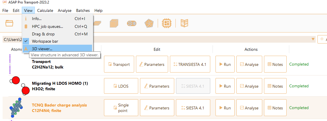
Alternatively, select a project a click View in the menu bar, then, click 3D viewer…

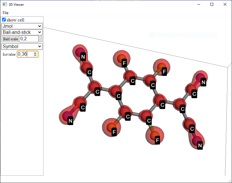
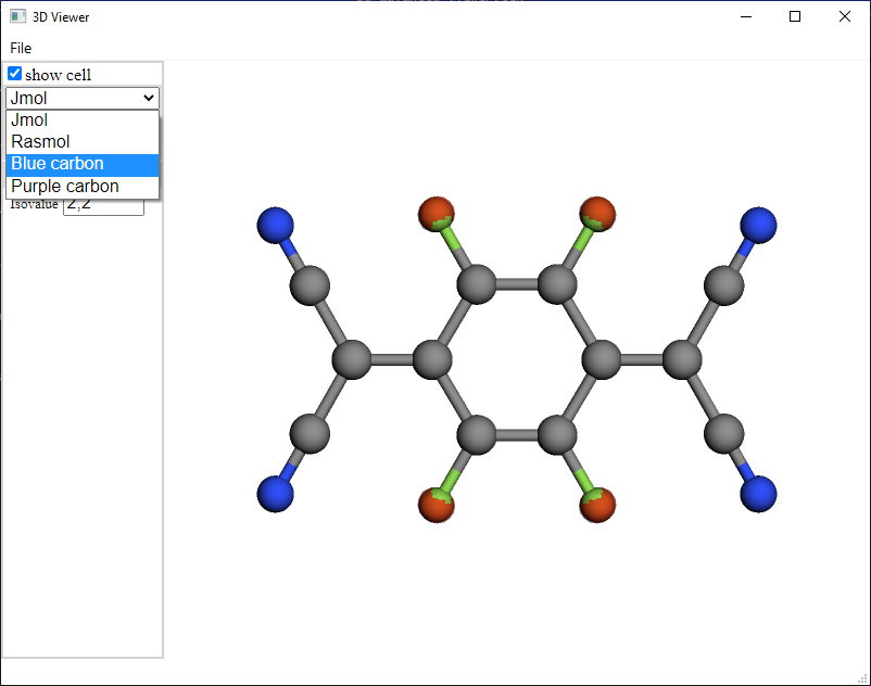
In the 3D viewer tab you can tune the following parameters:

• Appearance of the structure: Optionally Jmol or Rasmol representation style or blue/purple carbon atoms.

  

• Shape of atoms and bonds: Optionally balls and sticks, sticks and spheres.

  

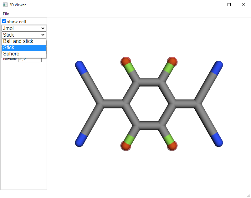
• Ball scale: Choose the scale of the balls that represent the atoms. The value 1 represents previously introduced Balls shape, 0 represents previously introduced Stick shape.

  

• Labels: It is specially useful to distinguish atoms by index or species.

  

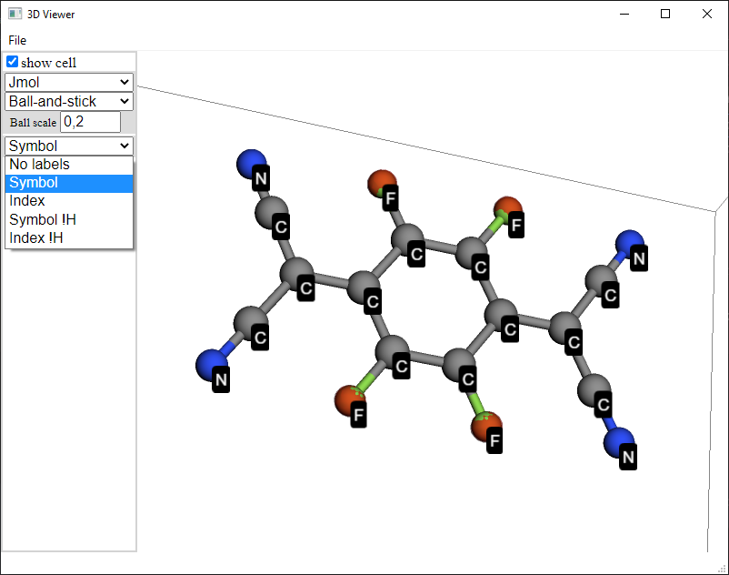
• Isovalue: To represent the surface that has the selected value of the electrostatic potential.