Parameters#
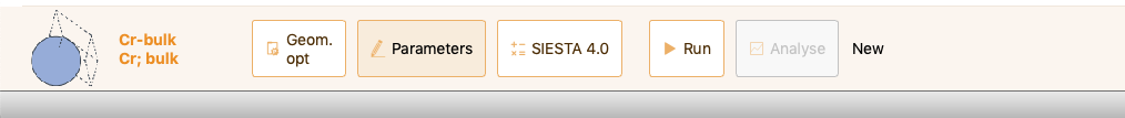
Select a project in the project tray, and click on the Parameters icon to open the Parameters widget.

You can use the Parameter widget to:
Set up the input parameters related to the different type of projects (Settings). See section Settings.
Edit the masses, magnetic moments and atomic positions of the system (Variables). See section Variables.
Set up the input parameters requiered to compute the target material properties of your calculation (Properties). See section Properties.
Settings#
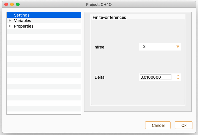
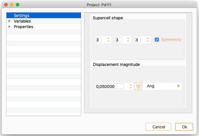
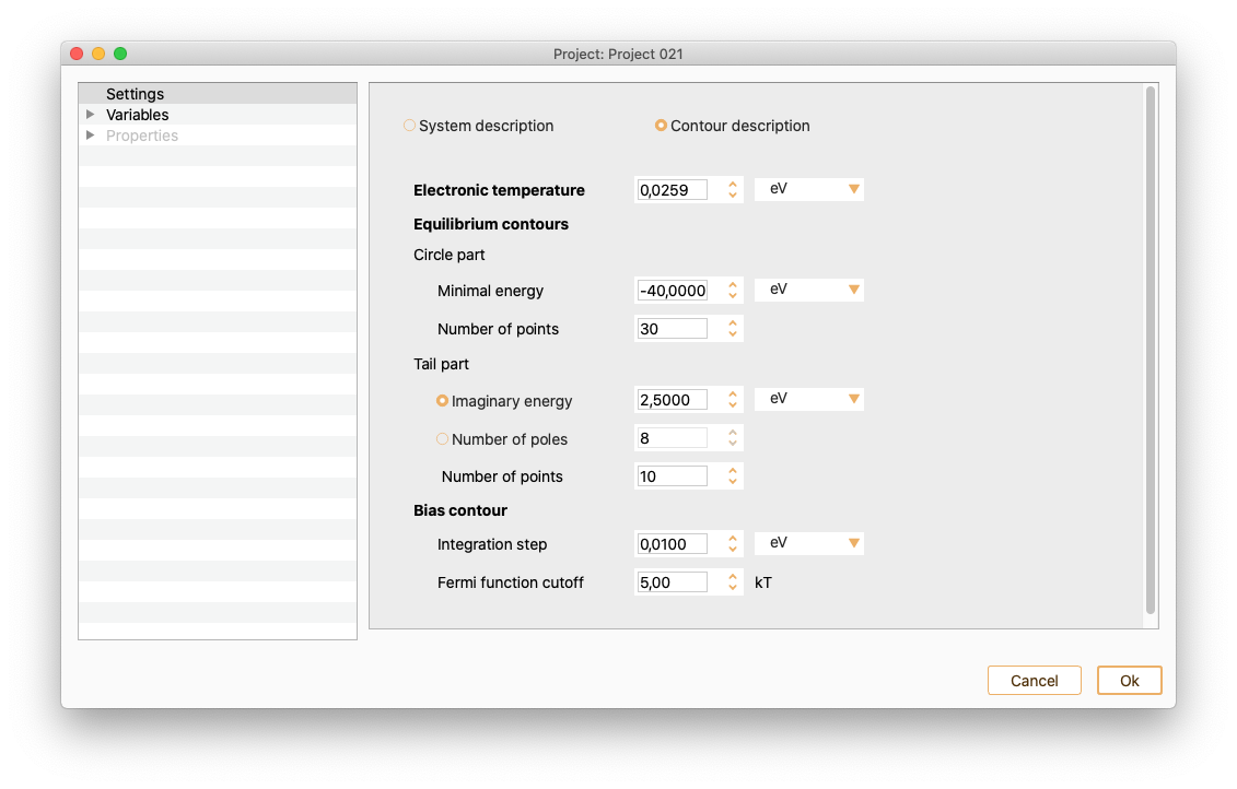
In the left side menu of the Parameters widget, select the Settings option. The input parameters you can introduce on this widget depend on the project type.
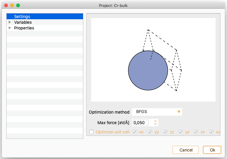
Geometry optimisation. See section Geometry Optimisation.
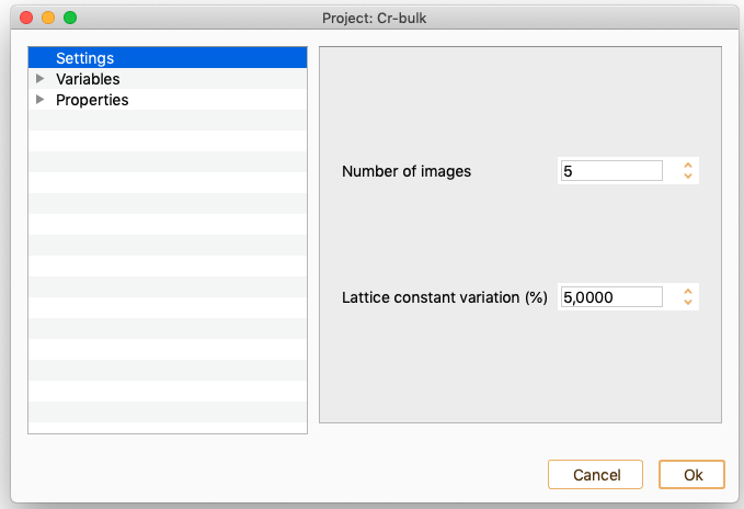
Equation Of State. See section Equation Of State (EOS).
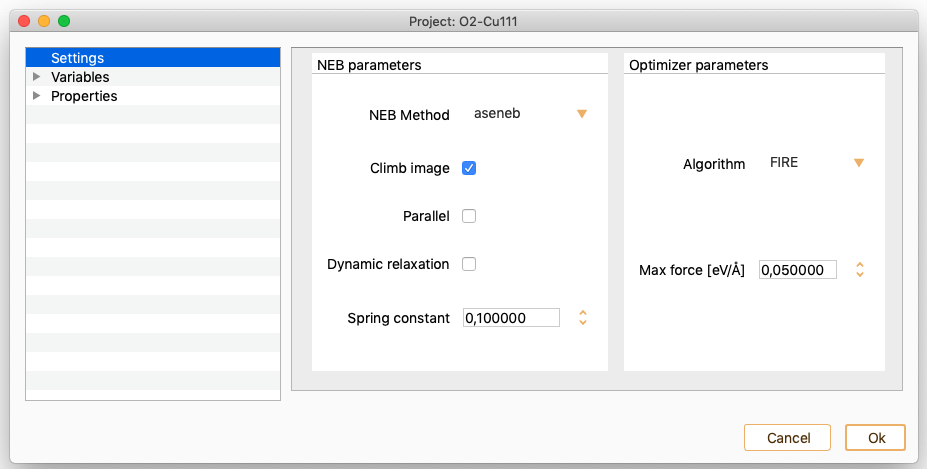
Nudged Elastic Band. See section Nudged Elastic Band (NEB).
Vibrations. See section Vibrations.
Phonons. See section Phonons.
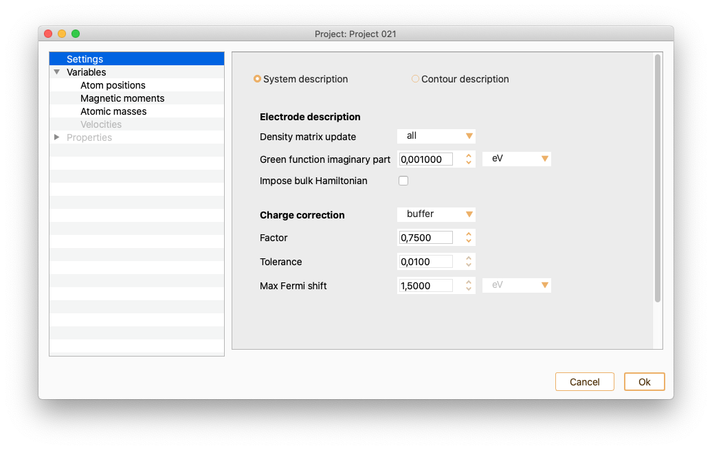
Electronic transport calculations. See section Electronic transport calculations.
Variables#
In the left side menu of the Parameters widget, select the Variables option. You can use it to edit widget atom positions, magnetic moments, atomic masses and velocities.
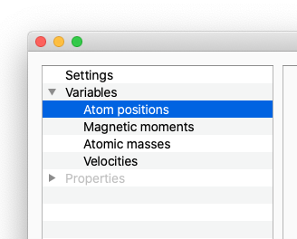
Atom positions
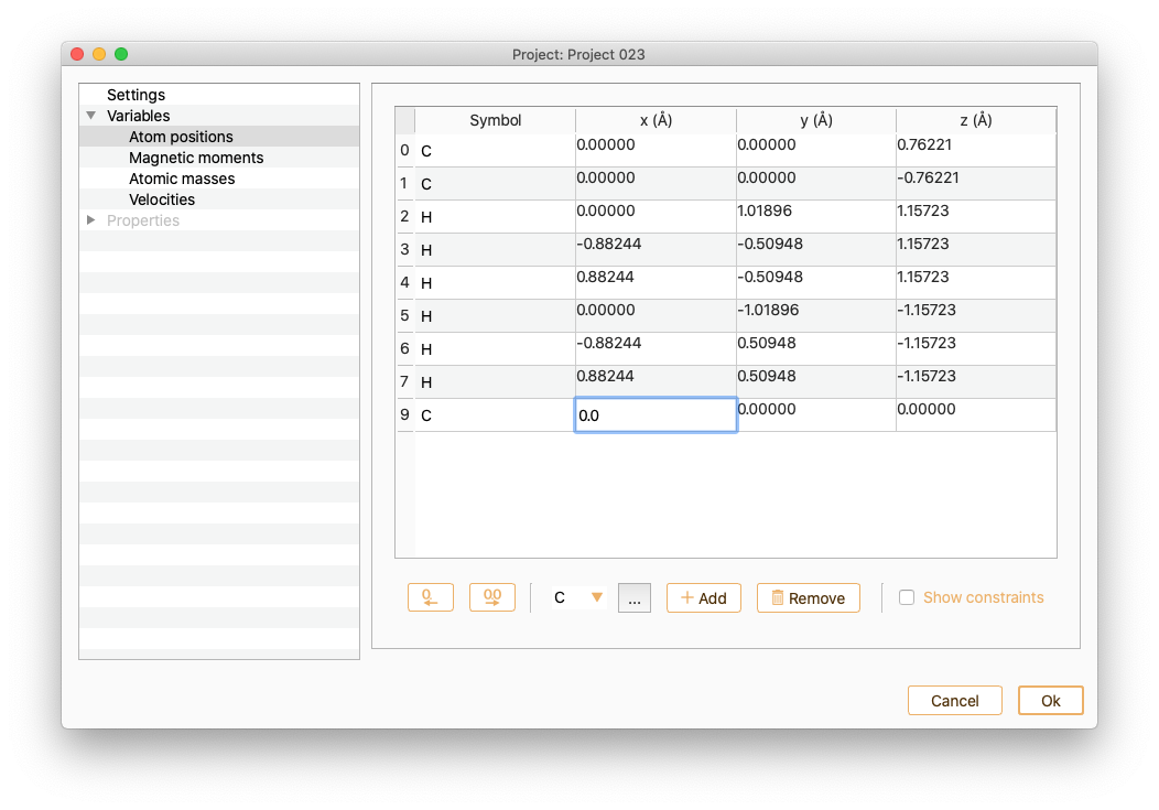
Select Atom positions to see information on the x, y and z coordinates (unit of Angström). Notice that the list of the atom indices starts at 0. You can change it to 1 by double-clicking in the index column.
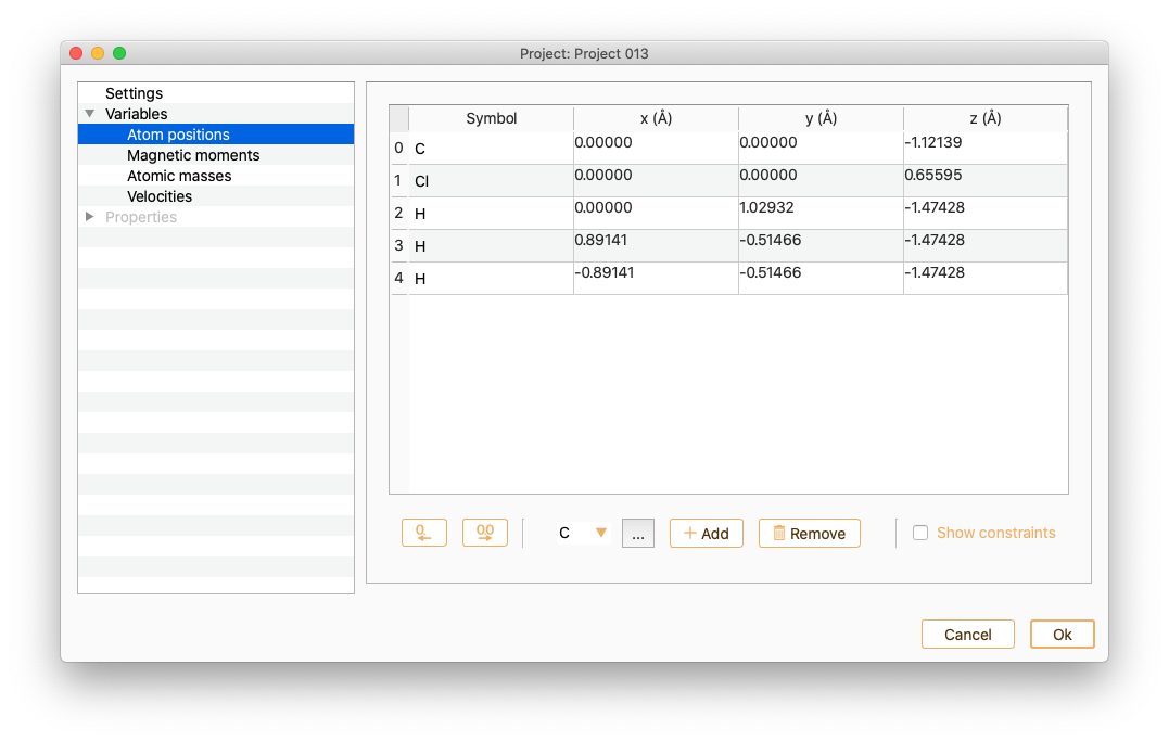
You can also use this widget to edit the atomic positions.
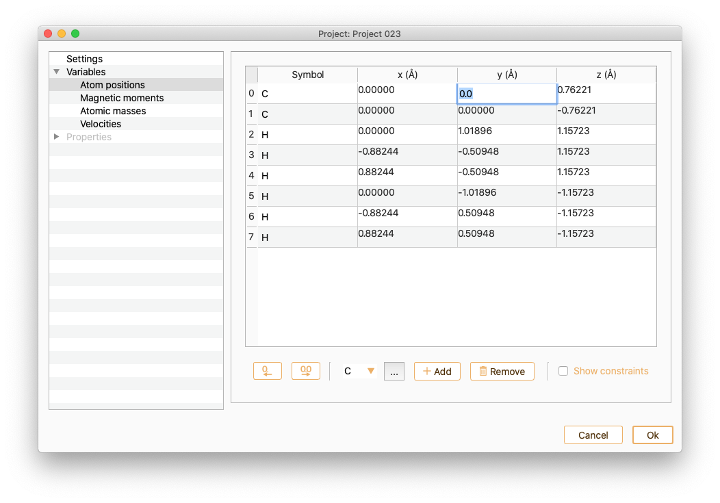
To add a new atom to the atomic structure, specify first the symbol of the chemical element and then press the Add atom button. Or click the … button to choose the chemical element from the dialog list and then press the Add atom button.
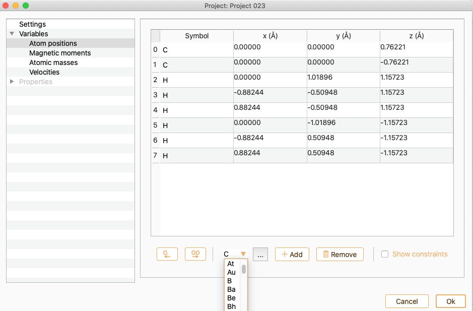
You can edit the atomic positions of the new atom.
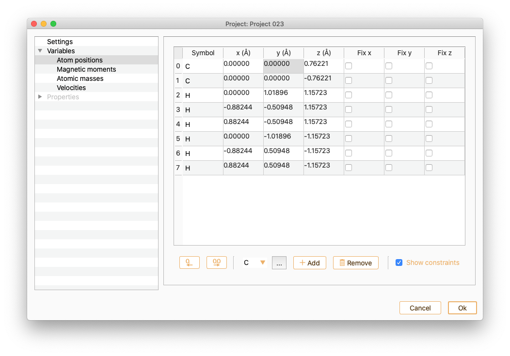
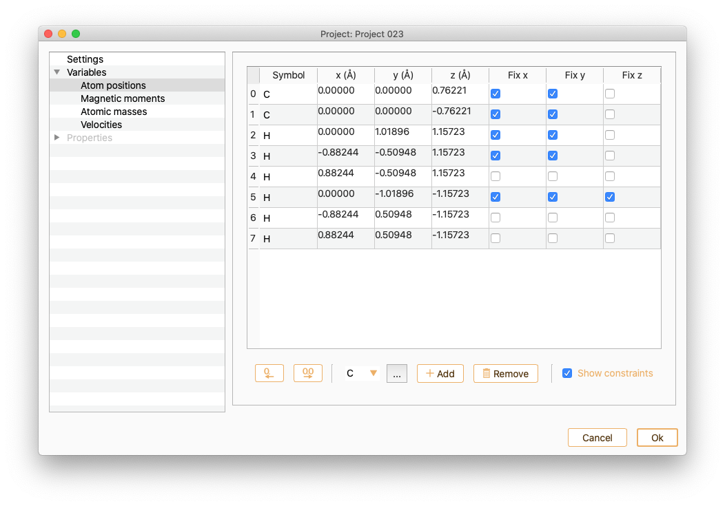
Click the Show constraints button to set up the constraints (i.e. keep some degrees of freedom in the system fixed). You can add constraints in any set of cartesian directions.
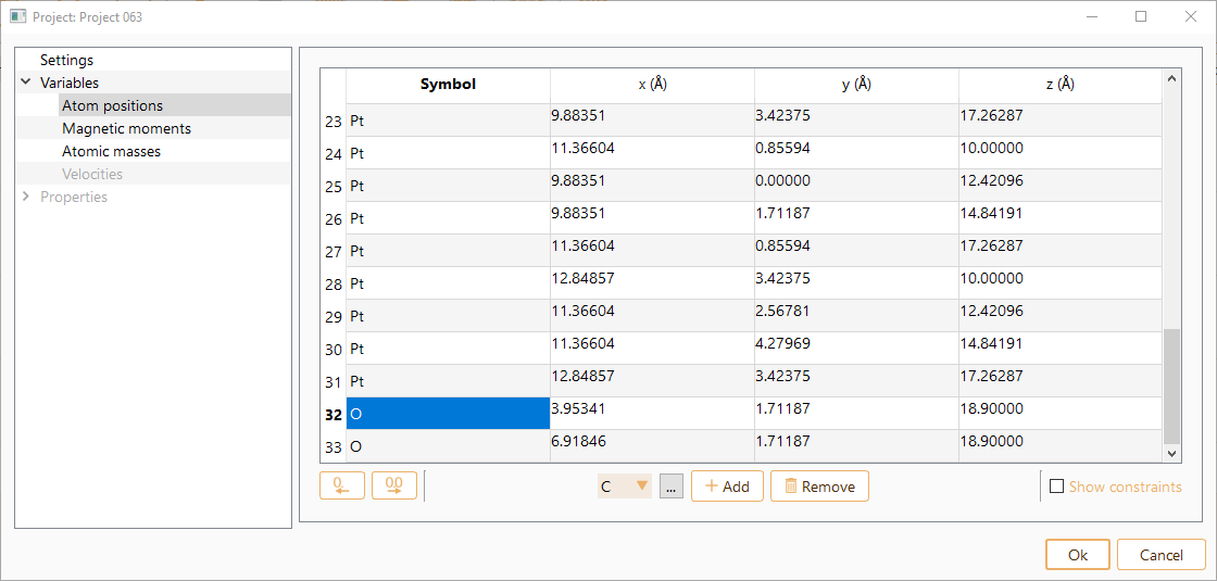
Note that you can drag and drop the rows to rearrange the order of atom indexes in the table:

Magnetic moments
Select the Magnetic moments variable to see and edit the magnetic moment of the atoms.
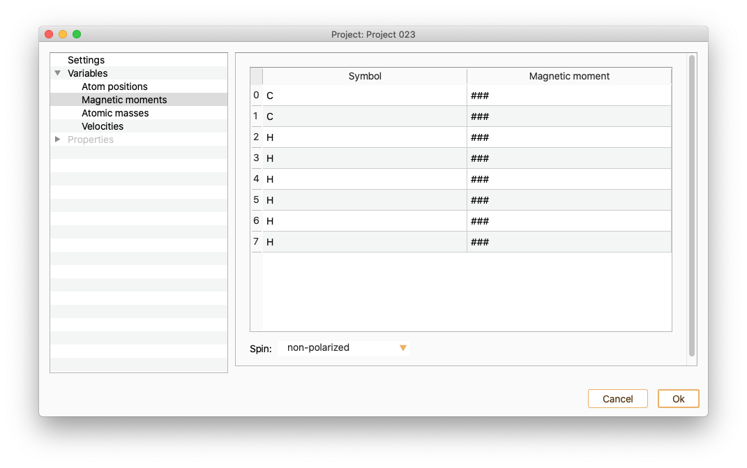
Open the Spin Dialog to modify the polarisation of your system.
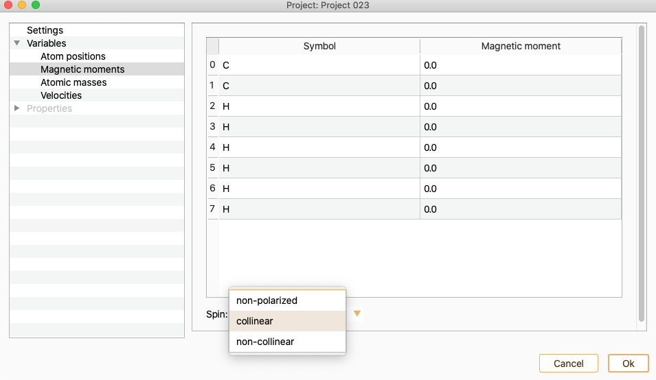
The available options are:
collinear. To perform a calculation with collinear spin (two spin components).
non-collinear. To perform a calculation with non-collinear spin (four spin components), up-down and angles.

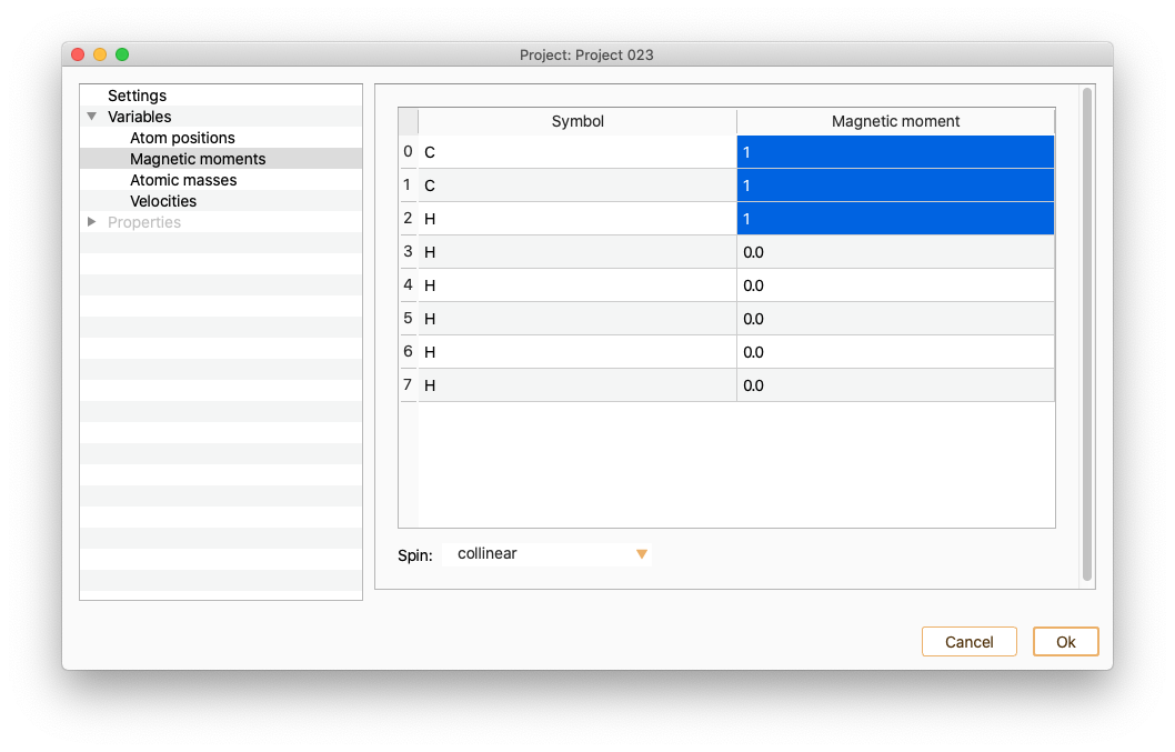
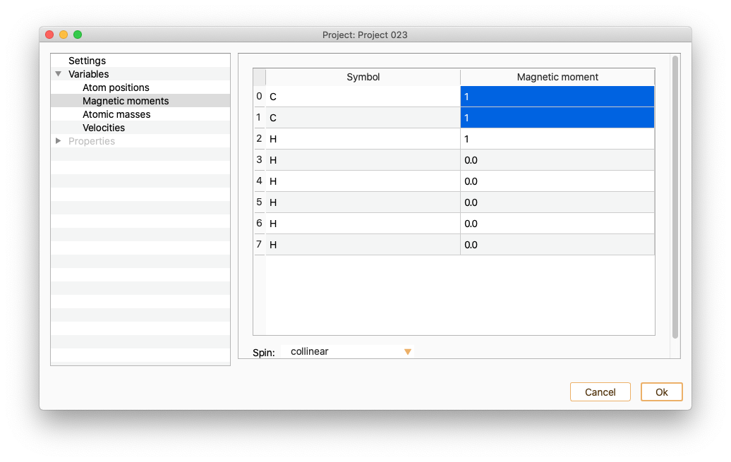
To set the magnetic moment of a set of atoms to a specific value, select in the magnetic moment column of all of them and edit one of the values. The magnetic moment of the rest of the selected atoms will be automatically set to the same value.
Moreover, it is possible a batch selection/deselection of atoms according to their chemical species by double-clicking in the Symbol column.
Atomic masses
The table contains information on atom index, atomic symbol and mass (atomic mass Unit) for each of the atoms in your system. You can edit the mass of any of the atoms on the list.
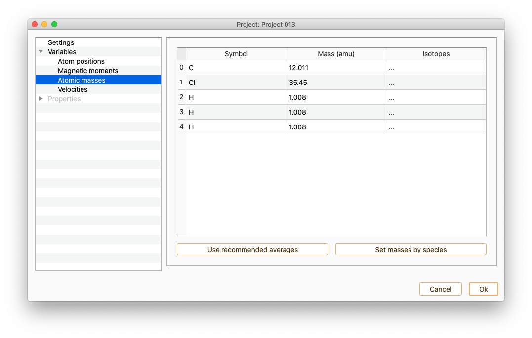 Click the Use recommended averages button to set the recommended average masses for each atom. By default these values will be chosen. It can be changed one by one double-clicking on the Mass column.In order to change the masses of all the atoms of the same chemical species at once, press the Set masses by species button.
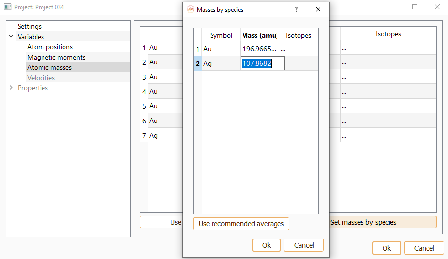
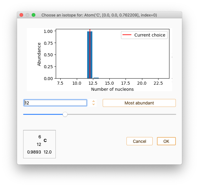
Use double-click on the field labelled Isotopes if you want to choose an isotope for the selected atom.
Velocities
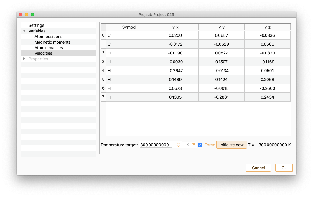
This variable option is only available in the Molecular Dynamics project type. (See section Molecular Dynamics.)After selecting Velocities you can see the information on the x, y and z coordinates (velocity unit Ang/fs).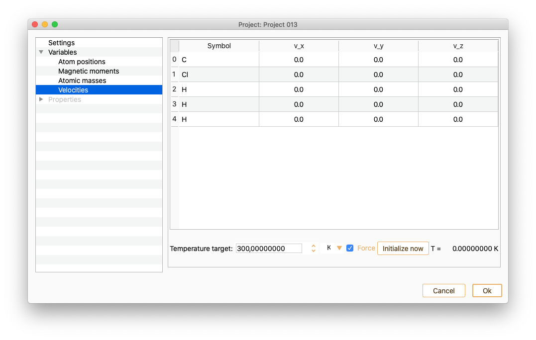 Notice that the list of atom indices start at 0. Tune the Temperature target (in units of K, eV or meV) to change the velocities.Enabling or diabling the Force option.
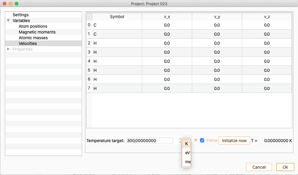
To visualise the velocity changes, press Initialize now buttom.
Properties#
In the left side menu of the Parameters widget, select the Properties option. Then, you can edit the parameters required to compute the target electronic material properties of your calculation. We indicate below the material properties that can be computed with ASAP. In parentheses, we indicate the calculator available to compute each of them:
- Electronic Density Of States (DOS) and Projected Density Of States (PDOS)
(SIESTA, Quantum ESPRESSO)
Band structure (SIESTA, Quantum ESPRESSO)
Charge (SIESTA)
Bader Charge (SIESTA)
Electrostatic potential (SIESTA)
Fermi surface (SIESTA, Quantum ESPRESSO)
Electronic Density Of States and Projected Density Of States#
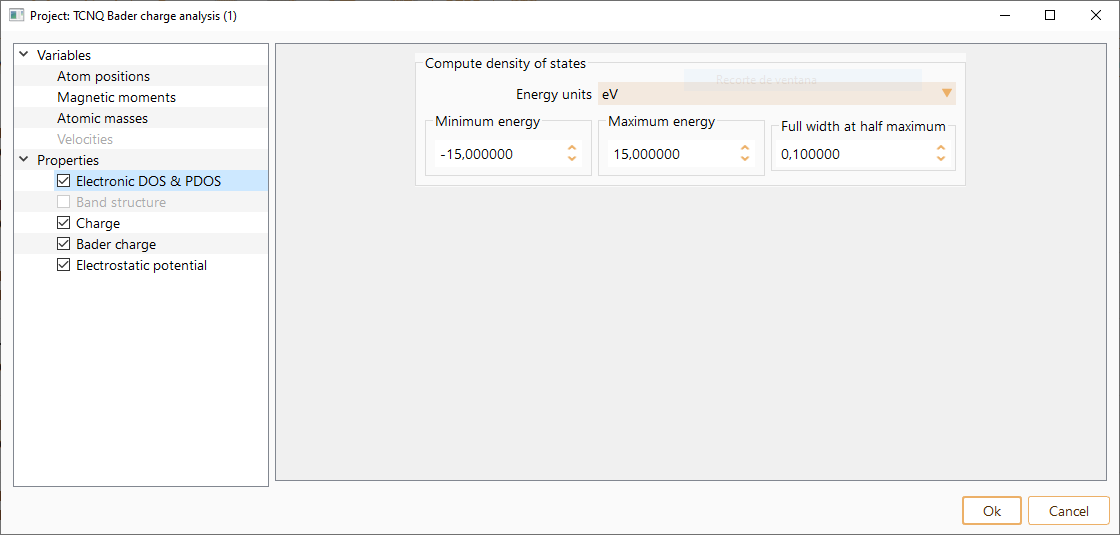
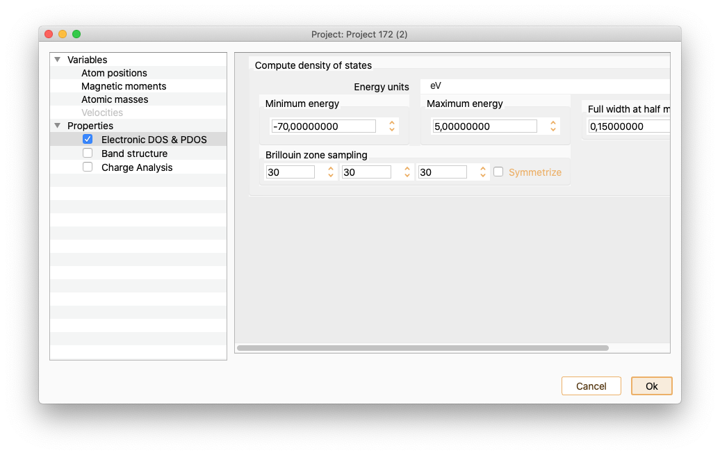
Click on the Electronic DOS :math:`&` POS Property to see the widget containing the parameters needed to compute DOS and PDOS.
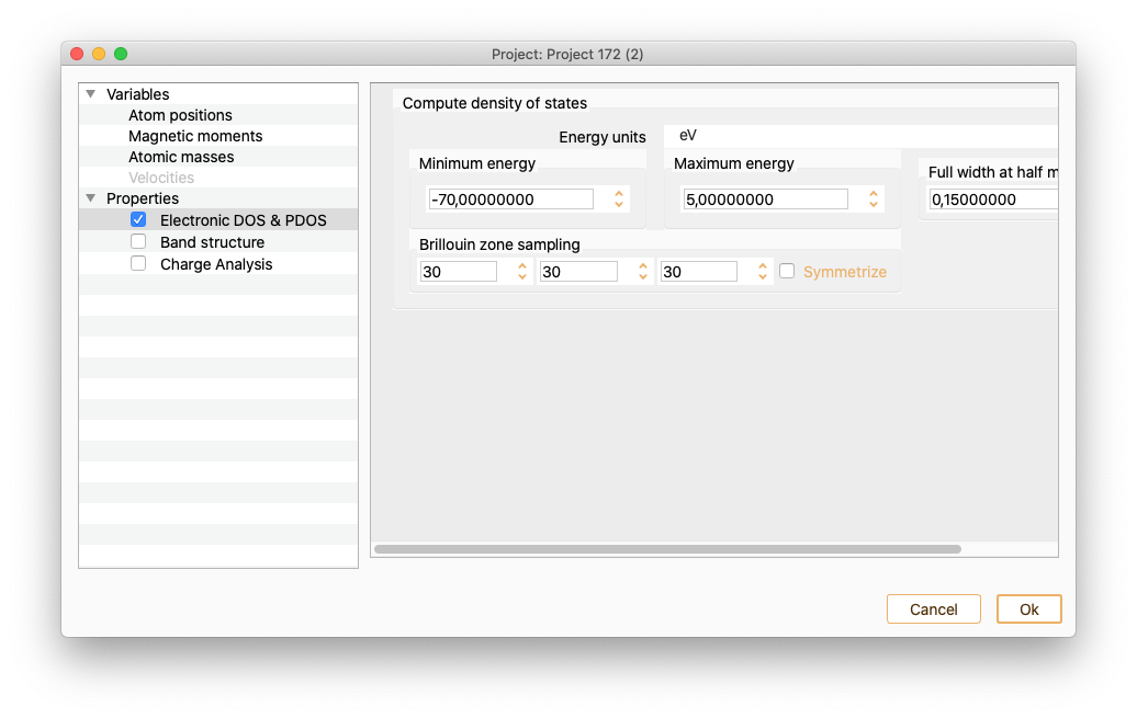
The widget has the following entries:
Energy units. To select the energy units.
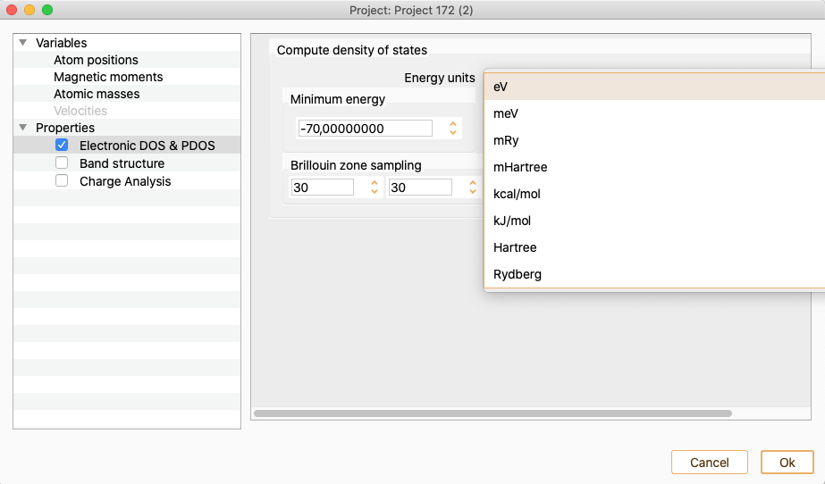
Minimum energy. Minimum energy at which DOS and PDOS will be evaluated.
Maximum energy. Maximum energy at which DOS and PDOS will be evaluated.
Full width at half maximum. It defines the smearing of the plotted curve. It is the width of the spectrum measured between points on the y-axis which are half the maximum amplitude.
Brillouin zone sampling. Number of k-points used to generate DOS and PDOS.
Press OK button to close the DOS and PDOS widget after the parameters are properly set.
Band structure#
Click on the Band Structure Property to open the band structure widget.
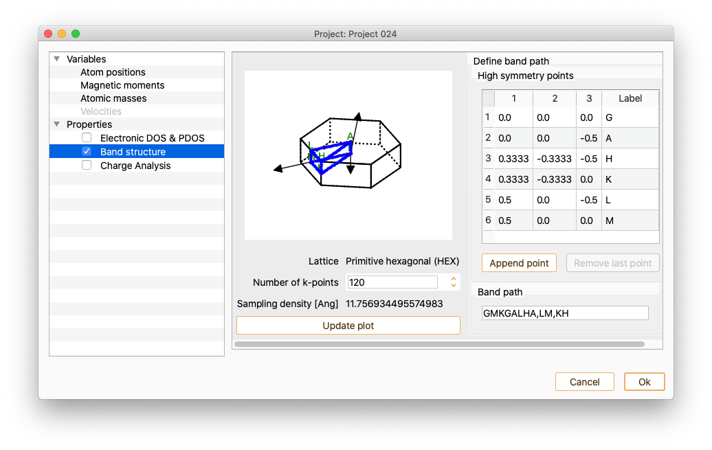
The lattice type is recognised for a few Bravais lattice types. In that case, several common k-points are labelled automatically. The automatic k-point labelling currently supports the following Bravais lattice types:
Primitive cubic
Face-centred cubic
Body-centred-cubic
Primitive tetragonal
Primitive hexagonal
Body centered tetragonal
Primitive orthorhomobic
Click the button Append point to add new k-points to the band path if desired.
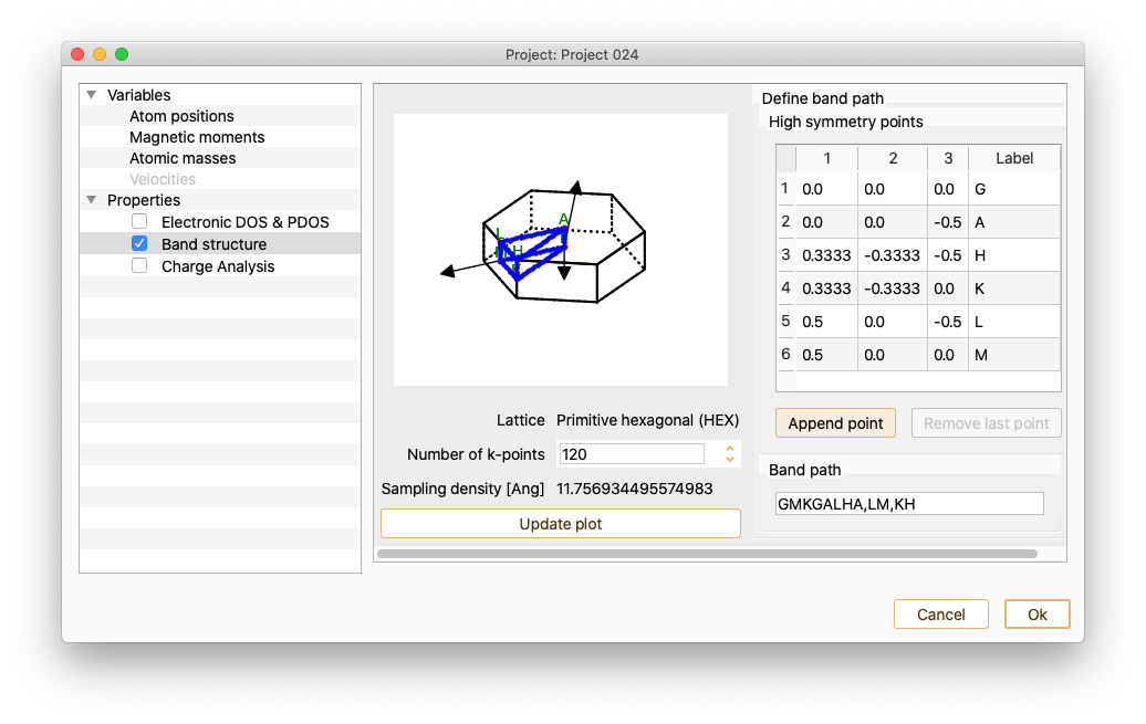
Use doble-click on each of the added k-points to edit k-point coordinates and label.
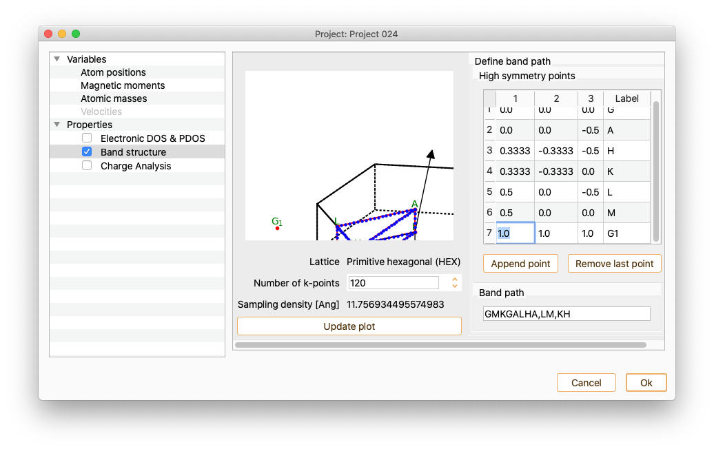
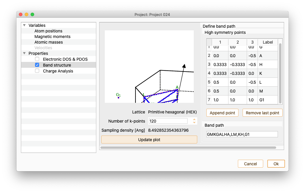
To incorporate the new labels to the path, add a string consisting of high-symmetric points labels in the field Band path.
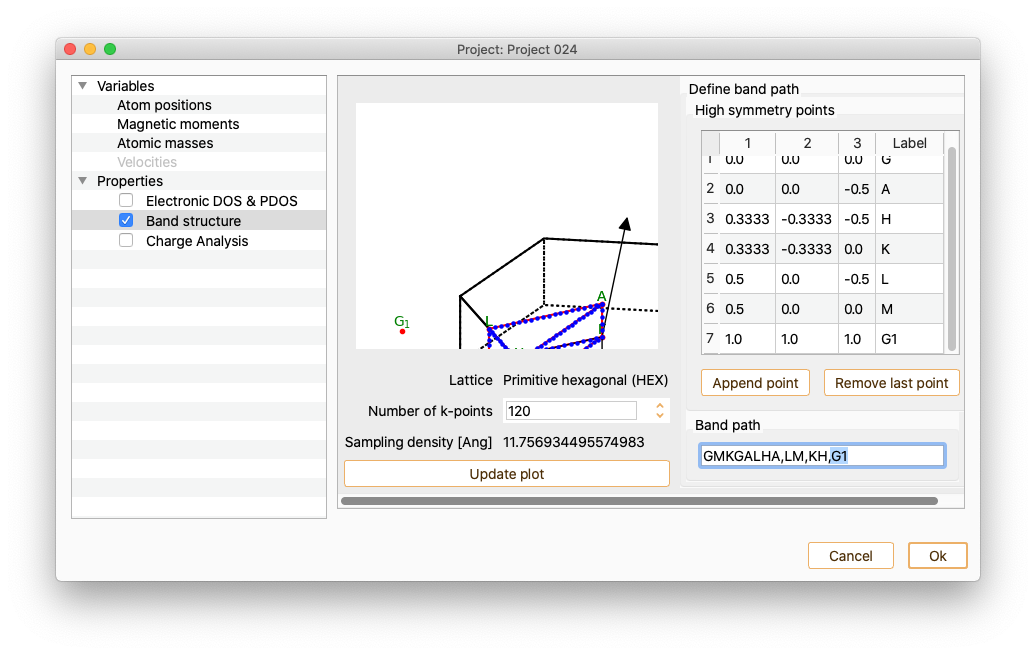
After pressing the Update plot button, the figure showing the unit cell’s Brillouin zone is automatically updated.
Local density of states#
Charge#
Click on the Charge Analysis Property to open the charge widget.
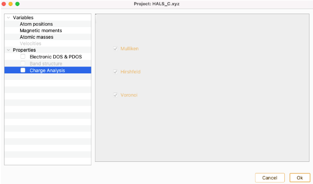
The assignment of charges to individual atoms is essentially arbitrary because the only charge that can be observed is the net charge of the whole molecule. ASAP implements three of the existing approaches to quantify atomic charges which are shown as check boxes.
- Mulliken: Mulliken method is based on populations of (atom-centered) basis function. For each atom, the contribution of all the electronic charge from the orbitals centered at one atom are combined and electronic overlap clouds between two atoms are divided equally to the two atoms. However, this distribution is erroneous if the atoms are different. Mulliken method also has a strong basis function dependency which means that changing the basis functions could make a big difference on the charges.This method should be used as a quick and qualitative overview.
Hirshfeld: The charge of each atom is obtained by integrating the electron density over its volume. The volumes are defined by constructing a promolecule, which is the superposition of spherically averaged electron densities of isolated atoms. In this method the volumes of the atoms overlap with each other.
- Voronoi (Voronoi deformation density): This method partitionates the space into non overlapping areas modeled as Voronoi cells. For each atom, the Voronoi cell of one atom is the region in space closer to the nucleus of that atom than to any other nucleus. These cells do not take into account the atomic size, although that does not impair the atomic charge.Then the charge of each atom is calculated by integrating the electron density over their respective Voronoi cell. The main difference between the Hirshfeld and Voronoi methods lies in the choice of the weight factor. Between them is preferable the Voronoi method in view of its simple definition of the atomic domain.
Bader charge#
The bader charge assigned to an atom represents the net charge associated with that atom within its AIM (Atoms In Molecules) region.
Click on the Bader charge property to see the corresponding parameters.
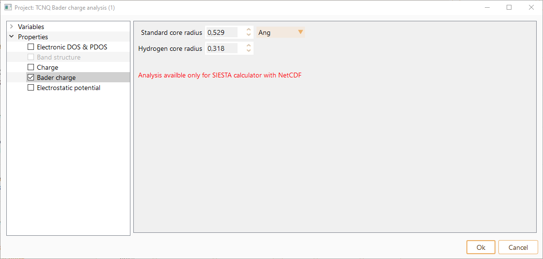
The bader charge assigned to an atom represents the net charge associated with that atom within its AIM (Atoms In Molecules) region. An atom is defined by the electronic charge density. In particular, the partitioning of the electrons is determined according to density zero-flux surfaces.
You can tune the following parameters, optionally in units of Ang, Bohr and nm.
Standard core radius: the distance from the nucleus of an atom within which the electron density is considered to be part of the atom’s core.
Hydrogen core radius: specific distance from the nucleus of a hydrogen atom within which the electron density is considered to be part of the hydrogen atom’s core.
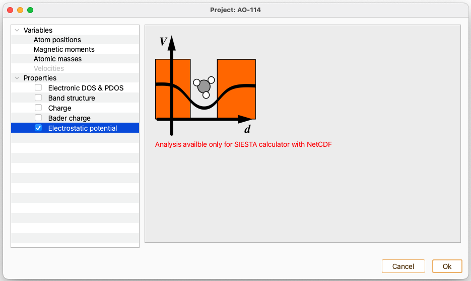
Electrostatic Potential#
Fermi Surface#
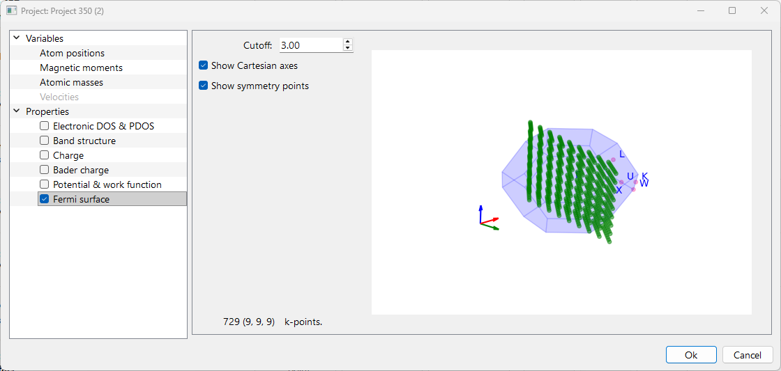
Cutoff: The cutoff option adjusts the resolution of the Fermi surface by controlling the density of k-points used in the calculation. Higher cutoff values result in a finer grid of k-points leads to a more detailed and accurate visualization. The corresponding k-point density is displayed in the right-side panel and updated dynamically.
Check the checkbox Show Cartesian Axes and Show Symmetry Points to display the Cartesian axes and symmetry points in the figure shown at right-side panel, respectively.